Overcoming Class Imbalance in Drug-Target Interaction Prediction: Strategies, Benchmarks, and Future Directions
Accurate prediction of Drug-Target Interactions (DTIs) is crucial for accelerating drug discovery, yet it is severely challenged by class imbalance, where known interacting pairs are vastly outnumbered by non-interacting ones.
Overcoming Class Imbalance in Drug-Target Interaction Prediction: Strategies, Benchmarks, and Future Directions
Abstract
Accurate prediction of Drug-Target Interactions (DTIs) is crucial for accelerating drug discovery, yet it is severely challenged by class imbalance, where known interacting pairs are vastly outnumbered by non-interacting ones. This article provides a comprehensive resource for researchers and drug development professionals, exploring the foundational causes and impacts of this imbalance. It details a suite of computational solutions, from data-level resampling techniques like SMOTE and GANs to algorithm-level approaches such as cost-sensitive learning and specialized deep learning architectures. The content further offers practical guidance for troubleshooting model performance and presents a rigorous framework for validating and benchmarking new methods against established standards, ultimately outlining a path toward more robust and predictive computational models in biomedicine.
The Class Imbalance Problem: Why Drug-Target Interaction Prediction is Inherently Biased
Defining Between-Class and Within-Class Imbalance in DTI Datasets
Frequently Asked Questions
What is class imbalance in Drug-Target Interaction (DTI) prediction? In DTI datasets, class imbalance occurs when the number of confirmed interacting pairs (the positive or minority class) is much smaller than the number of non-interacting or unlabeled pairs (the negative or majority class). This is a fundamental challenge because standard classification models become biased toward the majority class, making them poor at identifying the rare, but crucial, interacting pairs [1] [2].
What is the difference between "Between-Class" and "Within-Class" imbalance? This is a critical distinction for diagnosing issues in your dataset:
- Between-Class Imbalance: This is the overall skew in the dataset, where the total number of negative samples far exceeds the total number of positive samples [1]. It is the most commonly recognized form of imbalance.
- Within-Class Imbalance: This is a more subtle issue where, even within a single class (e.g., the minority positive class), there is a significant disparity in the representation of different subtypes. For instance, in the positive class, interactions for certain types of proteins (like enzymes) may be well-represented, while interactions for others (like nuclear receptors) are very rare [1].
Why is a model with high accuracy potentially misleading for DTI prediction? On a severely imbalanced dataset, a naive model that simply predicts "no interaction" for every drug-target pair will achieve a very high accuracy because it is correct for the vast majority of samples. However, its performance on the minority class of interest (the interactions) will be zero. This is why accuracy is a poor metric, and you should rely on metrics like the F1-score, Precision, Recall, and Area Under the Precision-Recall Curve (AUPRC) [3].
What are the most common strategies to mitigate class imbalance? The two primary categories of solutions are:
- Data-Level Strategies: These involve modifying the training dataset to create a more balanced class distribution. This includes random undersampling of the majority class, random oversampling of the minority class, and advanced synthetic oversampling techniques like SMOTE [4] [3].
- Algorithm-Level Strategies: These involve modifying the learning algorithm itself to compensate for the imbalance. This can include using ensemble methods like BalancedBaggingClassifier [3], adjusting class weights in the model's loss function [5], or employing specialized deep learning architectures designed for imbalanced data [1] [6].
Troubleshooting Guides
Problem: My Model is Biased and Fails to Predict Any Interactions
Description After training, your model's predictions are skewed entirely towards the majority (non-interacting) class. It has effectively "given up" on learning to identify true drug-target interactions.
Diagnosis Steps
- Check Class Distribution: Calculate the ratio of negative to positive samples in your training set. A ratio higher than 10:1 indicates a severe between-class imbalance that requires intervention [1].
- Evaluate with Robust Metrics: Stop using accuracy. Instead, evaluate your model using a confusion matrix, precision, recall, and the F1-score for the positive class. A high accuracy with a recall of zero for the positive class confirms the bias [3].
- Perform EDA for Within-Class Issues: Cluster your positive samples based on protein family (e.g., Enzymes, GPCRs, Ion Channels) or drug properties. A highly uneven distribution among clusters signals a within-class imbalance problem [1].
Solutions
- For Between-Class Imbalance:
- Random Undersampling: Randomly remove samples from the majority class until the classes are balanced. This is computationally efficient but may discard potentially useful information [4] [3].
- Synthetic Oversampling (SMOTE): Generate new, synthetic examples for the minority class by interpolating between existing minority class instances. This creates a balanced dataset without simple duplication [3].
- Ensemble with Undersampling: To mitigate information loss from undersampling, train multiple deep learning models. In each model, keep all positive samples but use a different random subset of the negative samples. Then, aggregate the predictions [1].
- For Within-Class Imbalance:
- Cluster-Based Oversampling: Apply oversampling techniques (like SMOTE) not to the entire positive class, but separately within each underrepresented cluster of positive samples. This ensures all subtypes of interactions are adequately represented [1].
Table 1: Comparison of Data-Level Resampling Techniques
| Technique | Principle | Pros | Cons | Best For |
|---|---|---|---|---|
| Random Undersampling [4] [3] | Removes majority class examples at random. | Reduces dataset size, faster training. | Can discard useful data, potential loss of model performance. | Very large datasets where the majority class is vastly redundant. |
| Random Oversampling [4] [3] | Duplicates minority class examples at random. | Simple, no loss of information. | Can lead to overfitting due to exact copies of data. | Small datasets where the minority class is very small. |
| SMOTE [3] | Creates synthetic minority class examples via interpolation. | Increases diversity, reduces risk of overfitting. | May generate noisy samples if the feature space is complex. | Datasets with a moderately sized minority class and clear feature manifolds. |
| Ensemble + RUS [1] | Trains multiple models on different balanced subsets. | Mitigates information loss from undersampling. | Computationally more expensive. | Complex, high-value datasets where preserving all possible signals is critical. |
Problem: How to Systematically Design an Experiment to Address Imbalance
Description You need a reliable, reproducible protocol to test different imbalance mitigation strategies on your specific DTI dataset.
Experimental Protocol
1. Data Preparation and Feature Engineering
- Dataset: Use a standard benchmark like BindingDB [1] [2]. Define a binding affinity threshold (e.g., IC50 < 100 nM) to label positive and negative interactions [1].
- Feature Extraction:
- Splitting: Split the data into training (85%) and testing (15%) sets. Crucially, apply resampling techniques ONLY to the training set to avoid data leakage and obtain a realistic evaluation on the original, imbalanced test set [4].
2. Implement and Compare Strategies Train your chosen model (e.g., Random Forest, Deep Neural Network) on multiple versions of the training data:
- Baseline: The original, imbalanced training set.
- Strategy A: Training set after Random Undersampling.
- Strategy B: Training set after SMOTE oversampling.
- Strategy C: Training set after a combined approach (e.g., SMOTE followed by Tomek Links cleaning [4]).
3. Evaluation and Model Selection
- Evaluate all models on the same, untouched imbalanced test set.
- Use a table to compare key metrics. Prioritize Sensitivity (Recall) and F1-score for the positive class, as they are more informative than accuracy in this context [3]. The Area Under the ROC Curve (AUC-ROC) is also useful, but the Area Under the Precision-Recall Curve (AUPRC) is often more telling for imbalanced problems [1].
Table 2: Key Metrics for Evaluating DTI Models on an Imbalanced Test Set
| Metric | Formula / Principle | Interpretation in DTI Context |
|---|---|---|
| Sensitivity (Recall) | ( \frac{TP}{TP+FN} ) | The model's ability to correctly identify true drug-target interactions. A low value means many interactions are missed. |
| Precision | ( \frac{TP}{TP+FP} ) | The reliability of the model's positive predictions. A low value means many predicted interactions are false leads. |
| F1-Score | ( 2 \times \frac{Precision \times Recall}{Precision + Recall} ) | The harmonic mean of precision and recall. A single balanced metric to optimize for. |
| Specificity | ( \frac{TN}{TN+FP} ) | The model's ability to correctly identify true non-interactions. |
| AUC-ROC | Area under the Receiver Operating Characteristic curve. | Measures the model's overall ability to distinguish between classes across all thresholds. |
| AUPRC | Area under the Precision-Recall curve. | More informative than AUC-ROC when the positive class is rare; focuses on performance for the class of interest. |
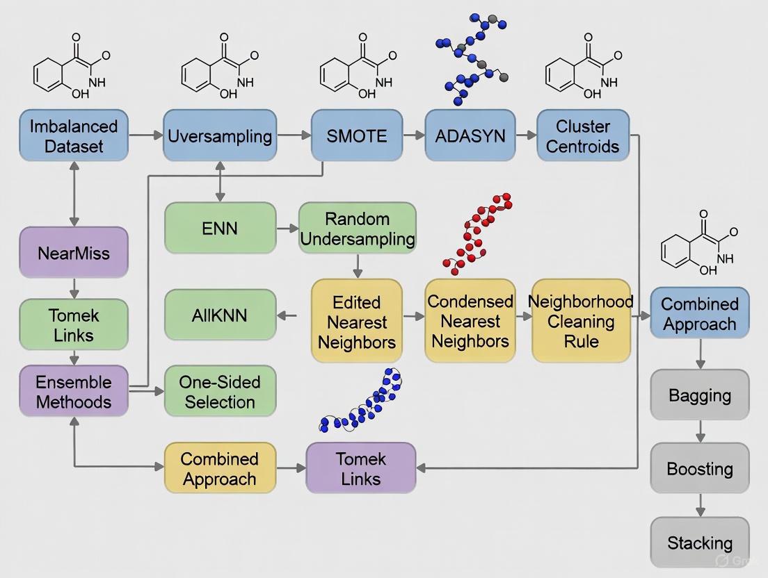
The following workflow diagram illustrates the complete experimental protocol for addressing class imbalance in DTI datasets.
The Scientist's Toolkit
Table 3: Essential Research Reagents and Computational Tools for DTI Imbalance Research
| Item Name | Type | Function / Description |
|---|---|---|
| BindingDB [1] [2] | Dataset | A public, curated database of measured binding affinities for drug-target pairs. Serves as the primary source for positive and negative interaction labels. |
| imbalanced-learn [4] [3] | Python Library | Provides a wide range of resampling techniques, including RandomUnderSampler, RandomOverSampler, and SMOTE, for easy implementation of data-level solutions. |
| MACCS Keys / ErG Fingerprints [1] [2] | Drug Feature | A method to encode the molecular structure of a drug compound into a fixed-length binary bit vector, representing the presence or absence of specific substructures. |
| Amino Acid / Dipeptide Composition [1] [2] | Target Feature | A simple yet effective method to represent a protein sequence by its relative composition of single amino acids or pairs of adjacent amino acids. |
| BalancedBaggingClassifier [3] | Algorithm | An ensemble method that combines bagging with internal resampling to balance the data for each base estimator, directly tackling the class imbalance. |
| F1-Score & AUPRC [1] [3] | Evaluation Metric | The critical metrics for evaluating model performance, focusing on the correct identification of the minority (interacting) class rather than overall accuracy. |
Why is Class Imbalance a Critical Problem in Drug-Target Interaction Prediction?
A: Class imbalance is a fundamental challenge in drug-target interaction (DTI) prediction because the number of known interacting pairs is vastly outnumbered by non-interacting pairs. This creates a significant bias in machine learning models, causing them to prioritize predicting "non-interaction" to achieve deceptively high accuracy, while performing poorly at identifying the rare but crucial "interacting" pairs, which are the primary focus of drug discovery [7] [8]. If unaddressed, this imbalance degrades the predictive performance for the minority class of interacting pairs, leading to more false negatives and hindering the identification of new drug candidates [9].
What Are the Typical Imbalance Ratios in Publicly Available DTI Databases?
A: The imbalance ratios in popular DTI databases are severe. The table below summarizes the documented statistics, which illustrate the scale of the challenge.
| Database | Total Interactions | Number of Drugs | Number of Targets | Documented Imbalance Ratio (Non-interacting : Interacting) |
|---|---|---|---|---|
| DrugBank (v4.3) | 12,674 [7] [8] | 5,877 [7] [8] | 3,348 [7] [8] | Not explicitly stated, but the ratio is inherently high due to the combinatorial possibility of drug-target pairs. |
| BindingDB (Various Affinity Measures) | Not Explicitly Stated | Not Explicitly Stated | Not Explicitly Stated | ~99:1 (Approximated from dataset characteristics used in research) [9] |
Experimental Context from Research:
Research utilizing the BindingDB database often curates specific datasets for DTI prediction. One such study using a dataset derived from BindingDB reported an extreme imbalance where non-interacting pairs outnumbered interacting pairs by a factor of approximately 99 to 1 [9]. This level of imbalance is a typical characteristic of real-world DTI data and poses a major obstacle for predictive modeling.
What Experimental Protocols Are Used to Quantify and Address This Imbalance?
A: Researchers employ specific computational workflows to first quantify the imbalance and then apply techniques to mitigate its effects. The following diagram illustrates a general experimental protocol for handling class imbalance in DTI prediction.
Detailed Methodologies for Key Steps:
1. Data Representation (Drug & Target Feature Extraction):
- Drug Features: Molecular structures are converted into fixed-length numerical vectors. Common methods include:
- MACCS Keys: A set of binary fingerprints (0/1) indicating the presence or absence of specific chemical substructures and functional groups [9].
- Molecular Descriptors: Software packages like
Rcpiin R are used to calculate constitutional, topological, and geometrical descriptors that capture various molecular properties [7] [8].
- Target Features: Protein sequences are also converted into numerical descriptors using tools like the PROFEAT web server. Computed features include [7] [8]:
- Amino acid composition.
- Dipeptide composition.
- Autocorrelation descriptors.
- Quasi-sequence-order descriptors.
2. Imbalance Handling Techniques:
- Data-Level - Generative Adversarial Networks (GANs): GANs are used to generate synthetic, but realistic, feature vectors for the minority class (interacting pairs). This artificially balances the dataset before training. A study using GANs with a Random Forest classifier on BindingDB data reported significant performance improvements, achieving accuracy over 97% [9].
- Algorithmic-Level - Ensemble Learning: This method involves creating multiple models. It first addresses between-class imbalance by using multiple balanced subset models of the majority class. It then tackles within-class imbalance (where some types of interactions are rarer than others) by using clustering to identify these "small disjuncts" and artificially enhancing them via oversampling to ensure the model learns these rare concepts [7] [8].
The Scientist's Toolkit: Research Reagent Solutions
| Tool / Resource | Type | Primary Function in DTI Research |
|---|---|---|
| DrugBank | Database | A comprehensive repository containing chemical, pharmacological, and pharmaceutical drug data along with comprehensive drug target information [7] [8]. |
| BindingDB | Database | A public database of measured binding affinities, focusing primarily on interactions between drug-like chemicals and proteins deemed to be drug targets [9]. |
| PROFEAT | Web Server | Computes a comprehensive set of numerical descriptors for proteins and peptides directly from their amino acid sequences, enabling machine learning applications [7] [8]. |
| Rcpi | R Package | An R toolkit for generating various types of molecular descriptors and structural fingerprints from drug compounds, facilitating drug-centric feature extraction [7] [8]. |
| Generative Adversarial Network (GAN) | Algorithm | A deep learning model used for data generation; in DTI, it creates synthetic data for the minority class to correct severe class imbalance [9]. |
In computational drug discovery, a model's high accuracy can be deceptive. A critical and often overlooked issue is class imbalance, where the number of inactive drug-target pairs in a dataset vastly outnumbers the active ones. This skew leads to models that are biased toward the majority class, failing to identify the rare but crucial active interactions that could lead to new therapies [10]. This technical guide addresses how to diagnose, troubleshoot, and resolve the problems caused by imbalanced data in your drug-target interaction (DTI) and drug-target affinity (DTA) prediction experiments.
Frequently Asked Questions
FAQ 1: My model has 95% accuracy, but my wet-lab team can't find any true active compounds. What's wrong?
Answer: High overall accuracy often masks poor performance on the minority class (active compounds) in imbalanced datasets. Standard accuracy is a biased metric when classes are skewed; a model can achieve over 90% accuracy by simply predicting "inactive" for every sample [11] [12]. This results in a high false negative rate, causing promising active compounds to be missed.
Solution:
- Use Robust Metrics: Replace accuracy with a suite of metrics that are sensitive to class imbalance.
- Prioritize: F1-score, Matthews Correlation Coefficient (MCC), and Area Under the Precision-Recall Curve (AUPR) [13] [12]. The table below summarizes key metrics to use.
| Metric | Description | Why Use It for Imbalanced Data? |
|---|---|---|
| F1-Score | Harmonic mean of precision and recall. | Balances the trade-off between finding all actives (recall) and ensuring predictions are correct (precision) [13]. |
| MCC | A correlation coefficient between observed and predicted classifications. | Considered a balanced measure that works well even on imbalanced datasets [13] [12]. |
| AUPR | Area under the Precision-Recall curve. | More informative than ROC-AUC when the positive class is rare [13]. |
| Balanced Accuracy | Average of recall obtained on each class. | Prevents over-optimistic estimates from the majority class [12]. |
FAQ 2: What are the most effective techniques to fix an imbalanced dataset for DTI prediction?
Answer: Both data-level and algorithm-level techniques are effective. Recent research indicates that random undersampling (RUS) of the majority class to a moderate imbalance ratio (e.g., 1:10) can be highly effective for highly skewed bioassay data [12].
Solution: A Comparison of Resampling Techniques The following table compares common resampling methods based on recent applications in cheminformatics.
| Technique | Method | Advantages | Disadvantages | Reported Performance |
|---|---|---|---|---|
| Random Undersampling (RUS) | Randomly removes majority class samples. | Simple, fast, can significantly boost recall & F1-score [12]. | Risks losing potentially useful data [10]. | Outperformed ROS and synthetic methods on highly imbalanced HIV, Malaria datasets [12]. |
| Synthetic Oversampling (SMOTE) | Creates synthetic minority class samples. | Mitigates overfitting from mere duplication [10]. | Can generate noisy samples; struggles with high dimensionality [10]. | Showed limited improvement in some DTI tasks; MCC lower than RUS in studies [12]. |
| NearMiss | Selectively undersamples majority class based on proximity to minority class. | Redizes computational cost and can improve recall [10] [12]. | Can discard critical majority class samples forming decision boundaries [10]. | Achieved highest recall but lowest precision and accuracy in validation [12]. |
FAQ 3: How can I ensure my model is fair and not biased against specific data subgroups?
Answer: Bias can manifest if a model performs well overall but poorly for a specific subset of targets or drug classes. Evaluating fairness metrics is essential for robust scientific models.
Solution:
- Define Facets: Identify potential subgroups in your data (e.g., different protein families or compound structural classes).
- Calculate Fairness Metrics: Use libraries like
AIF360orFairlearnto compute metrics such as Demographic Parity and Equal Opportunity [14]. - Interpretation: These metrics help answer questions like, "Does my model have an equal true positive rate across different protein families?" ensuring that predictive performance is equitable across the biological landscape [11] [14].
Troubleshooting Guides
Problem: Model is Overconfident and Unreliable in Real-World Screening
Explanation: Traditional deep learning models for DTI prediction often lack the ability to quantify uncertainty. They may produce a high prediction score for a novel drug-target pair that is actually outside the model's knowledge, leading to wasted experimental resources on false positives [13].
Solution: Implement Uncertainty Quantification (UQ)
- Method: Integrate Evidential Deep Learning (EDL) into your model architecture.
- Experimental Protocol:
- Modify the Output Layer: Replace the standard softmax output with a layer that parameterizes a Dirichlet distribution.
- Change the Loss Function: Use a loss function like the Dirichlet loss, which penalizes incorrect and uncertain predictions.
- Calculate Uncertainty: The model's output includes both a predictive probability and an uncertainty estimate (e.g., the entropy of the Dirichlet distribution).
- Application: In a framework like EviDTI, this allows the model to express "I don't know" for out-of-distribution samples. Predictions can then be prioritized by confidence, dramatically increasing the hit rate in experimental validation [13].
Problem: Poor Performance on New Drugs or Targets (The Cold-Start Problem)
Explanation: Models trained on imbalanced data often generalize poorly, especially for novel drugs or targets with no known interactions in the training set [13] [15].
Solution: Leverage Self-Supervised Pre-training
- Method: Use models pre-trained on large, unlabeled molecular and protein sequence databases (e.g., ProtTrans for proteins, MG-BERT or ChemBERTa for drugs) [13] [15] [16].
- Experimental Protocol:
- Feature Extraction: Use the pre-trained model to generate rich, contextual representations for all drugs and targets in your dataset.
- Transfer Learning: Fine-tune a downstream classifier (e.g., a simple neural network) on your smaller, labeled DTI dataset using these pre-trained features.
- Benefit: This approach provides the model with a strong foundational understanding of molecular and protein linguistics, helping it make better predictions on novel entities, even with limited labeled data [15]. The workflow below illustrates this process.
Experimental Workflow for Handling Imbalanced DTI Data
The following diagram illustrates a robust workflow that integrates the solutions discussed above to build a reliable DTI prediction model.
The Scientist's Toolkit
| Research Reagent / Tool | Type | Function in Experiment |
|---|---|---|
| SMOTE / ADASYN | Software Algorithm | Generates synthetic samples of the minority class to balance datasets [10] [12]. |
| Random Undersampling (RUS) | Software Algorithm | Randomly removes samples from the majority class to achieve a desired imbalance ratio [12]. |
| Pre-trained Models (ProtTrans, ChemBERTa) | Software Library | Provides high-quality, contextual feature representations for proteins and drugs, improving model generalization [13] [16]. |
| Evidential Deep Learning (EDL) | Modeling Framework | Provides uncertainty estimates for predictions, allowing researchers to prioritize high-confidence candidates [13]. |
| Fairlearn / AIF360 | Software Library | Contains metrics and algorithms for assessing and improving fairness of models across subgroups [14]. |
| MCC (Matthews Correlation Coefficient) | Evaluation Metric | A single, balanced metric for evaluating classifier performance on imbalanced data [13] [12]. |
FAQs on Handling TWSNI in Drug-Target Interaction Prediction
What is a "Target with Few Known Interactions" and why is it a problem? A Target with Few Known Interactions (TWSNI) is a protein for which very few, or sparse, drug-target interactions have been experimentally confirmed [17]. This creates a significant "within-class imbalance" problem in machine learning. Unlike targets with many known interactions (TWLNI), TWSNI do not provide enough positive samples (known interactions) for a model to learn meaningful patterns, leading to poor prediction performance for these important but understudied targets [17].
What is the core computational strategy for improving TWSNI predictions? The most effective strategy is to use a different classification method for TWSNI than for TWLNI. For TWSNI, models must leverage information from "neighbor" targets—those that are biologically similar—by using the positive interaction samples from these neighbors to compensate for the lack of its own data [17]. This approach is a key part of multiple classification strategy methods like MCSDTI [17].
Beyond data-level fixes, what algorithmic approaches can help?
Using ensemble methods that are inherently more robust to class imbalance is beneficial. The BalancedBaggingClassifier is a prime example, as it combines bagging (bootstrap aggregating) with additional balancing during the training of each individual model in the ensemble [3]. This ensures that each classifier pays adequate attention to the minority class. Furthermore, adjusting class weights in your model to increase the penalty for misclassifying the rare TWSNI interactions can also improve performance [18].
Which evaluation metrics should I avoid and which should I use for TWSNI models? You should avoid using accuracy as a primary metric, as it is highly misleading with imbalanced data [18] [3]. Instead, use metrics that are sensitive to the performance on the minority class:
- Precision: Measures how many of the predicted TWSNI interactions are correct.
- Recall: Measures how many of the actual TWSNI interactions you managed to find.
- F1-score: The harmonic mean of precision and recall, providing a single balanced metric [18] [3].
- AUC-ROC: Measures the model's ability to distinguish between interacting and non-interacting pairs across all thresholds and is insensitive to class imbalance [18].
What are the key differences in handling TWLNI vs. TWSNI?
| Feature | Targets with Larger Numbers of Interactions (TWLNI) | Targets with Smaller Numbers of Interactions (TWSNI) |
|---|---|---|
| Core Problem | Abundant positive samples [17] | Severe lack of positive samples (within-class imbalance) [17] |
| Primary Strategy | Predict interactions using their own sufficient data [17] | Predict interactions by leveraging data from similar "neighbor" targets [17] |
| Key Challenge | Sparsity of interactions in the drug-target pair space [17] | Positive samples are too few for a model to learn from effectively [17] |
| Independent Evaluation | Crucial to evaluate separately from TWSNI to see true performance [17] | Crucial to evaluate separately from TWLNI to prevent their results from being overwhelmed [17] |
Experimental Protocols for TWSNI Prediction
Protocol 1: Implementing the MCSDTI Framework
This protocol is based on the MCSDTI method, which uses multiple classification strategies [17].
1. Objective: To accurately predict drug-target interactions for both TWLNI and TWSNI by applying tailored classification strategies to each group.
2. Materials & Data Preprocessing:
- Datasets: Use established DTI datasets such as Nuclear Receptors (NR), Ion Channels (IC), GPCRs, or Enzymes (E) [17].
- Data Partitioning: Calculate the number of known interactions per target. Rank targets and split them into two groups:
- TWSNI: Targets with a number of interactions below a defined threshold (e.g., the median or a percentile).
- TWLNI: Targets with interactions above this threshold.
- Feature Extraction: For each drug-target pair, generate meaningful features. For drugs, this is often derived from their SMILES strings or molecular graphs. For targets, this is derived from their amino acid sequences or other protein descriptors [15].
3. Methodology:
- For TWLNI: Train a standard classifier (e.g., Random Forest, Gradient Boosting) using only the known interactions for each specific TWLNI. The ample data for these targets makes this feasible [17].
- For TWSNI:
- Step 1 - Find Neighbors: For each TWSNI, identify a set of biologically similar "neighbor" targets based on protein sequence similarity or functional similarity.
- Step 2 - Aggregate Data: Pool the known positive interaction samples from the TWSNI with those from its identified neighbors to create an augmented training set.
- Step 3 - Train Model: Train a classifier on this augmented dataset to predict interactions for the specific TWSNI [17].
4. Independent Evaluation:
- Evaluate the prediction performance for TWLNI and TWSNI separately. This prevents the overall results from being dominated by the easier-to-predict TWLNI and provides a clear view of how well the method handles the challenging TWSNI [17].
Protocol 2: A Workflow for Handling Imbalanced DTI Data
This general protocol outlines steps to address class imbalance at both the data and algorithmic levels [18] [3].
1. Objective: To build a robust DTI prediction model that effectively identifies potential interactions for minority-class targets (TWSNI).
2. Data Resampling:
- Technique: Apply the Synthetic Minority Over-sampling Technique (SMOTE).
- Procedure: Use the
imblearnlibrary in Python. SMOTE generates synthetic examples for the minority class (TWSNI interactions) by interpolating between existing minority class instances, rather than simply duplicating them [18] [3].
3. Algorithmic Approach:
- Technique: Use a Balanced Bagging Classifier.
- Procedure: Implement an ensemble model that combines the strengths of bagging with built-in balancing. This classifier trains multiple base estimators (e.g., Decision Trees) on balanced bootstrap samples of the data [3].
4. Model Evaluation:
- Metrics: Calculate Precision, Recall, F1-score, and AUC-ROC on the test set [18] [3].
- Analysis: Use a confusion matrix to visually inspect the true positives, false positives, true negatives, and false negatives, focusing on the model's performance on the minority TWSNI class [18].
Methodologies & Workflow Visualizations
MCSDTI Classification Strategy
This diagram illustrates the core decision process of the MCSDTI framework for handling different types of targets.
Multi-task Self-Supervised Learning for Cold Start
This diagram outlines the pre-training approach used by advanced frameworks like DTIAM to generate better representations for drugs and targets, which is particularly useful in cold-start scenarios like TWSNI.
The Scientist's Toolkit: Key Research Reagent Solutions
| Research Reagent / Tool | Function & Explanation |
|---|---|
| MCSDTI (Multiple Classification Strategy) | A computational framework that splits targets into TWSNI and TWLNI, applying a customized classification strategy for each group to optimize prediction [17]. |
| DTIAM | A unified framework that uses self-supervised learning on large amounts of unlabeled drug and target data to learn robust representations, improving predictions for DTI, binding affinity, and mechanism of action, especially in cold-start situations [15]. |
| SMOTE | A data-level technique that generates synthetic examples for the minority class (TWSNI interactions) to balance the dataset and reduce model bias [18] [3]. |
| BalancedBaggingClassifier | An ensemble algorithm that combines multiple base classifiers, each trained on a balanced bootstrap sample of the original data, making it inherently suited for imbalanced classification [3]. |
| Pre-training Models (Self-Supervised) | Models trained on large corpora of unlabeled molecular graphs and protein sequences. They learn general, powerful representations that can be fine-tuned for specific DTI tasks with limited labeled data, directly addressing the TWSNI data scarcity problem [15]. |
| F1-Score & AUC-ROC | Critical evaluation metrics that provide a truthful assessment of model performance on imbalanced datasets, focusing on the successful identification of the minority TWSNI class rather than misleading overall accuracy [18] [3]. |
A Toolkit of Solutions: From Data Resampling to Advanced Deep Learning
Frequently Asked Questions (FAQs)
FAQ 1: Why are data-level strategies like SMOTE or GANs necessary in drug-target interaction (DTI) prediction? In DTI prediction, the number of known interacting drug-target pairs (positive class) is vastly outnumbered by the number of non-interacting pairs (negative class). This is known as between-class imbalance [8]. Without correction, machine learning models become biased towards predicting the majority class (non-interacting), leading to poor performance in identifying therapeutically valuable interactions. Data-level strategies directly address this by synthetically creating new examples of the minority class to balance the dataset.
FAQ 2: My model has high accuracy but fails to predict any true drug-target interactions. What is happening? This is a classic symptom of class imbalance. Accuracy is a misleading metric when data is skewed. A model that simply predicts "non-interacting" for all examples will still achieve a high accuracy but is practically useless [19] [20]. You should switch to evaluation metrics that are more robust to imbalance, such as Precision, Recall, F1-Score, AUC-ROC, and especially AUC-PR [19] [20]. Furthermore, ensure you are using techniques like stratified sampling during train-test splits to preserve the class distribution in your validation sets [19].
FAQ 3: What is the fundamental difference between SMOTE/ADASYN and GANs for generating synthetic data? SMOTE and ADASYN are relatively simple, non-learned interpolation techniques. They create new data points by linearly combining existing minority class instances [21]. GANs, on the other hand, are deep learning models that learn the underlying probability distribution of the minority class data. Through an adversarial training process, they can generate highly realistic and novel synthetic data that can be more diverse than SMOTE-generated data [22].
FAQ 4: When should I consider using GANs over SMOTE for my DTI dataset? Consider GANs when:
- You have a sufficiently large and complex dataset, and you need to generate highly diverse and novel molecular structures [22].
- Advanced SMOTE variants (e.g., Borderline-SMOTE, SVM-SMOTE) still do not yield satisfactory performance.
- You have the computational resources and expertise to train a complex deep-learning model. For many standard applications, starting with SMOTE or one of its variants is recommended due to its simplicity and computational efficiency.
FAQ 5: After applying SMOTE, my model's performance on the independent test set did not improve. Why? This can occur due to several reasons:
- Overfitting on Synthetic Data: The model may have learned the specific patterns of the synthetically generated points, which do not generalize well to real-world data.
- Introduction of Noisy Samples: If synthetic instances are created in regions of the feature space that overlap with the majority class, they become "noisy" examples that confuse the classifier [21].
- Improper Application of SMOTE: SMOTE should only be applied to the training data after splitting. If you apply it to the entire dataset before splitting, you will cause data leakage, as information from the test set influences the training process, leading to over-optimistic and invalid performance estimates [4].
Troubleshooting Guides
Problem: The synthetic data generated by SMOTE is causing overfitting.
Explanation: SMOTE generates synthetic data by linear interpolation between neighboring minority class instances. This can lead to the creation of overly simplistic and redundant samples if the minority class has a complex distribution or contains noise, causing the model to learn a non-generalizable decision boundary.
Solution Steps:
- Use Advanced SMOTE Variants: Switch from vanilla SMOTE to more sophisticated versions designed to mitigate this issue.
- Borderline-SMOTE: This method only generates synthetic samples for minority instances that are misclassified by a k-Nearest Neighbors classifier (the "danger" instances). This focuses the data generation on the class boundary where it is most needed [21].
- SVM-SMOTE: This uses a Support Vector Machine (SVM) to identify support vectors (which often lie near the decision boundary) and generates synthetic data near these points [21].
- KMeans-SMOTE: This first clusters the minority class, then allocates more synthetic samples to sparse clusters, ensuring a more balanced distribution across the minority class [21].
- Combine Sampling with Cleaning: Use hybrid methods like SMOTE-Tomek. The Tomek Links method identifies and removes overlapping examples from both classes after SMOTE application, which can help in refining the class boundary and reducing noise [4].
- Validate Rigorously: Use nested cross-validation to more robustly evaluate the model's performance and tune hyperparameters, ensuring that the reported performance is not biased by overfitting.
Problem: My dataset includes both numerical and categorical features (e.g., molecular fingerprints), and SMOTE fails.
Explanation: Standard SMOTE operates in continuous feature space and uses Euclidean distance, making it incompatible with categorical data. Applying it directly to such mixed data will produce meaningless interpolated values for categorical features.
Solution Steps:
- Use SMOTE-NC (SMOTE-Nominal Continuous): This is an extension of SMOTE specifically designed to handle datasets with both numerical and categorical features. For a mixed-type feature vector, SMOTE-NC calculates the median of the standard deviations of all numerical features. It then uses this value in the distance calculation to find k-nearest neighbors. When generating a new sample, it copies the most frequent category among the k-nearest neighbors for the categorical columns [21].
- Alternative: Feature Engineering: Consider transforming your categorical features into a numerical representation that captures their relationships, if possible, though this is often non-trivial in chemical informatics.
Problem: The generative AI model (e.g., GAN) produces invalid molecular structures.
Explanation: GANs, particularly those generating molecular structures as SMILES strings or graphs, can sometimes output sequences that do not correspond to valid, syntactically correct, or chemically stable molecules.
Solution Steps:
- Use Domain-Specific Generative Models: Employ generative models specifically designed for molecular generation, such as REINVENT4. These models incorporate chemical knowledge and rules into the generation process, leading to a much higher rate of valid molecules. For instance, one study showed that a character-level RNN produced only 3% valid molecules, while REINVENT4 achieved 100% validity [22].
- Implement Validity Checks: Integrate a post-processing step that filters out invalid SMILES strings using a chemical validation toolkit like RDKit.
- Reinforcement Learning (RL) Fine-tuning: Fine-tune the generative model using RL with a reward function that penalizes invalid structures and rewards desirable chemical properties [22].
Comparative Analysis of Synthetic Data Strategies
The table below summarizes the key characteristics, advantages, and limitations of SMOTE, ADASYN, and GANs.
Table 1: Comparison of Data-Level Strategies for Handling Class Imbalance
| Feature | SMOTE | ADASYN | GANs |
|---|---|---|---|
| Core Principle | Interpolates between random minority class instances [21]. | Interpolates between instances, weighted by learning difficulty; focuses on "hard-to-learn" examples [20]. | Learns data distribution via adversarial training between generator and discriminator networks [22]. |
| Data Generation | Linear interpolation in feature space. | Linear interpolation, density-biased. | Non-linear, can model complex distributions. |
| Diversity of Data | Limited to convex combinations of existing data. | Limited to convex combinations, but more focused. | High potential for creating novel, diverse samples. |
| Computational Cost | Low [4]. | Low to Moderate. | Very High [22]. |
| Ease of Implementation | High (e.g., via imbalanced-learn). |
High (e.g., via imbalanced-learn). |
Low (requires deep learning expertise). |
| Handling of Within-Class Imbalance | No (treats all minority instances equally). | Yes (adaptively generates more data for harder examples). | Yes (can learn the full distribution, including rare sub-concepts). |
| Key Advantage | Simple, effective, and fast. Good starting point. | Can improve recall by focusing on difficult regions. | Can generate highly realistic and novel data. |
| Key Challenge | Can generate noisy samples in overlapping regions; ignores within-class imbalance [21]. | Can over-emphasize outliers. | Training instability; mode collapse; high resource demands [22]. |
Table 2: Quantitative Performance in Drug Discovery Contexts
| Method / Scenario | Key Performance Metric | Result | Context & Notes |
|---|---|---|---|
| Generative AI (REINVENT4) | Model Specificity on HTS Test Set (1:76 imbalance) | Improved from 0.08 to 0.56 [22] | Screening a large compound library; critical for reducing false positives. |
| Generative AI (REINVENT4) | ROC AUC on Scaffold Split Test | Improved from 0.72 to 0.81 [22] | Tests generalizability to novel chemical scaffolds. |
| Generative AI (REINVENT4) | G-Mean | Improved from 0.60 to 0.76 [22] | Geometric mean of sensitivity & specificity; good for imbalanced data. |
| FastUS (Undersampling) | AUC / F1-Score | Outperformed 4 state-of-the-art methods [8] | Highlights that sophisticated sampling can outperform simple random sampling. |
| Weighted Loss Function | Matthews Correlation Coefficient (MCC) | Can achieve high MCC, but less consistent than oversampling [23] | An algorithm-level strategy for comparison; performance can be volatile. |
Experimental Protocols
Protocol 1: Implementing SMOTE and its Variants for a DTI Dataset
This protocol outlines the steps to apply SMOTE and its advanced variants using the imbalanced-learn library in Python.
Objective: To balance an imbalanced DTI training set to improve classifier performance on the minority (interacting) class.
Materials (The Scientist's Toolkit):
- Software: Python with
imbalanced-learn(imported asimblearn),scikit-learn,pandas,numpy. - Data: A feature matrix (X) and label vector (y) for your DTI problem, split into training and testing sets.
Procedure:
- Data Preprocessing and Splitting:
- Perform necessary cleaning, normalization, and feature scaling on your dataset.
- Split the data into training and testing sets using stratified splitting (
train_test_splitwithstratify=y) to maintain the original imbalance ratio in the splits [19].
- Apply SMOTE (or variant) to Training Set Only:
- Crucially, apply the sampling technique only to the training data to prevent data leakage [4].
- For Standard SMOTE:
- For Borderline-SMOTE:
- Train Model and Evaluate:
- Train your chosen classifier (e.g., LightGBM, Random Forest) on the resampled training data (
X_train_resampled,y_train_resampled). - Make predictions on the original, unmodified test set (
X_test,y_test). - Evaluate performance using metrics like Precision, Recall, F1-Score, and AUC-PR.
- Train your chosen classifier (e.g., LightGBM, Random Forest) on the resampled training data (
The following diagram illustrates this workflow:
Workflow for Applying SMOTE
Protocol 2: A Generative AI Framework for Non-Active Compound Generation
This protocol is based on a published study that used generative models to address the scarcity of non-active compounds for GPCR targets [22].
Objective: To generate novel, valid non-active compounds for a specific protein target (e.g., M1 muscarinic receptor) to enhance the training set for a classification model.
Materials (The Scientist's Toolkit):
- Data Sources: Public bioactivity databases (ChEMBL, BindingDB, PubChem).
- Generative Models: CharRNN or more advanced models like REINVENT4.
- Validation Tools: Chemical validation toolkits (e.g., RDKit), clustering algorithms (e.g., for diversity analysis).
- Computing: Access to GPU resources for efficient model training.
Procedure:
- Data Curation:
- Collect known active and non-active compounds for your target from databases. Apply a clear activity threshold (e.g., ≤1μM for active, ≥10μM for non-active).
- Perform Tanimoto similarity analysis to ensure a clear structural distinction between active and non-active sets.
- Model Selection and Training:
- Select a generative model. The study found REINVENT4 vastly superior to CharRNN, producing 100% valid molecules compared to only 3% [22].
- Train the selected model on the curated set of known non-active compounds to learn their structural and physicochemical patterns.
- Generation and Validation:
- Use the trained model to generate a large number of candidate non-active molecules.
- Filter the generated molecules for chemical validity and desired properties.
- Perform clustering analysis (e.g., using Taylor-Butina clustering) to assess the structural diversity of the generated set compared to the original data.
- Model Enhancement:
- Incorporate the validated, generated non-active compounds into the training data for a DTI classifier.
- Re-train the classifier and evaluate its performance on a challenging external test set, such as a scaffold-split set or a high-throughput screening (HTS) dataset with a high imbalance ratio.
The following diagram illustrates this high-level framework:
Generative AI for Data Augmentation
Foundations: Tackling Class Imbalance in Drug Discovery
In computational drug discovery, the datasets used for training classification models, such as those predicting whether a compound is active against a biological target, are typically highly unbalanced. The number of inactive compounds vastly outnumbers the number of active substances. This class imbalance causes standard machine learning models to be biased toward the majority (inactive) class, leading to poor predictive performance for the critical minority (active) class you are often most interested in identifying [23].
Algorithm-level approaches directly modify machine learning algorithms to mitigate this bias. Unlike data-level methods (e.g., oversampling) that alter the training dataset, algorithm-level techniques preserve the original data distribution, maintaining its full informational content [24]. The two primary algorithm-level strategies are:
- Cost-Sensitive Learning (CSL): This strategy introduces distinct misclassification costs for each class during training. The underlying assumption is that a higher misclassification cost is assigned to samples from the minority class, forcing the model to pay more attention to them. The objective is to minimize the overall high-cost errors [24] [25].
- Ensemble Methods: These methods combine multiple base models to create a more robust and accurate classifier. When tailored for class imbalance, they often integrate principles from CSL or resampling techniques to strengthen the collective prediction for the minority class [24].
Troubleshooting Cost-Sensitive Learning
FAQ: What is the core principle behind Cost-Sensitive Learning? CSL operates on the principle that not all prediction errors are equal. Misclassifying a rare, active compound (a false negative) is more detrimental to a drug discovery campaign than misclassifying a common, inactive one (a false positive). CSL algorithms formalize this by assigning a higher penalty or cost to errors made on the minority class. The model's training objective then becomes the minimization of total cost, rather than total errors, which improves its ability to identify the critical class [24].
FAQ: I've implemented a cost-sensitive model, but I'm getting too many false positives. How can I refine the cost matrix? An excess of false positives indicates that the cost assigned to the minority class might be disproportionately high, causing the model to become overly sensitive. The following troubleshooting guide addresses this and other common issues.
| Problem | Potential Cause | Recommended Solution |
|---|---|---|
| High False Positive Rate | Cost for minority class is set too high, making the model overly sensitive. | Systematically reduce the cost assigned to the minority class and re-evaluate performance using metrics like Precision and F1-score [25]. |
| Poor Generalization (Overfitting) | The cost matrix is over-optimized for the training set, learning its noise. | Validate your cost matrix on a separate validation set or using cross-validation. Consider using a robust method like a Random Undersampling Ensemble (RUE) to feedback a more generalizable error rate for cost assignment [25]. |
| Persistent High False Negatives | Assigned costs for the minority class are still too low to overcome the data imbalance. | Increase the cost weight for the minority class. Explore advanced "personalized cost assignment" strategies that assign different costs to different instances based on their location information rather than a constant cost for the entire class [25]. |
Experimental Protocol: Implementing a Cost-Sensitive Random Forest A common and effective way to apply CSL is using a cost-sensitive variant of the Random Forest algorithm. Below is a detailed methodology based on common practices in the field [12].
- Data Preparation: Start with your pre-processed drug-target interaction dataset (e.g., molecular fingerprints and target features). Split the data into training, validation, and test sets, ensuring the imbalance ratio is consistent across splits.
- Baseline Model Training: Train a standard Random Forest classifier on the training set without any cost adjustments. This provides a performance baseline.
- Assign Class Weights: Implement CSL by calculating class weights. A standard method is to set the class weight to be inversely proportional to the class frequencies. For example, using the "balanced" mode in libraries like scikit-learn, where the weight for a class is given by:
weight = total_samples / (n_classes * count_of_class_samples). - Train Cost-Sensitive Model: Train a new Random Forest model on the same training set, but this time incorporate the calculated class weights. This tells the algorithm to penalize misclassifications of the rare class more heavily.
- Evaluation and Comparison: Evaluate both the baseline and cost-sensitive models on the validation set. Use metrics robust to imbalance, such as Matthews Correlation Coefficient (MCC), F1-score, and Balanced Accuracy. The cost-sensitive model should show a marked improvement, particularly in recall for the minority class and MCC [23] [12].
Troubleshooting Ensemble Methods: Rotation Forest
FAQ: Why is the Rotation Forest algorithm particularly effective for imbalanced drug data? Rotation Forest is an ensemble method that aims to build accurate and diverse classifiers. It works by randomly splitting the feature set into subsets, performing Principal Component Analysis (PCA) on each subset, and then reconstructing a full feature space for training a base classifier (like a decision tree). This process enhances both the accuracy and diversity of the individual classifiers in the ensemble. For imbalanced data, this diversity is crucial as it allows the ensemble to capture complex patterns associated with the minority class that a single model might miss [26]. Its performance can be further boosted by hyperparameter optimization and feature selection [26].
FAQ: My Rotation Forest model is computationally expensive. How can I optimize it? The process of multiple PCA transformations is inherently more computationally intensive than simpler ensembles like Random Forest. To optimize it:
- Feature Selection: Prior to training, apply feature selection techniques (like Sequential Forward Selection or Exhaustive Feature Selection) to reduce the dimensionality of the data. This directly reduces the PCA computation load [26].
- Hyperparameter Tuning: Use efficient hyperparameter optimization frameworks like Optuna with the Tree-structured Parzen Estimator (TPE) sampler. This intelligently explores the hyperparameter space (e.g., number of subsets, base estimators) to find a high-performance configuration with fewer trials [26].
Experimental Protocol: Building an Optimized Rotation Forest Model This protocol outlines the steps for creating a high-performance Rotation Forest model, incorporating hyperparameter tuning and feature selection as described in recent research [26].
- Data Preprocessing: Normalize or standardize your dataset (e.g., the Breast Cancer Coimbra dataset with clinical biomarkers) to ensure that the PCA step in Rotation Forest is not dominated by features on different scales.
- Hyperparameter Optimization with Optuna:
- Define an objective function that trains a Rotation Forest model with a given set of hyperparameters (e.g., number of estimator subsets, PCA components).
- Use the F1-score on the training data (or via cross-validation) as the optimization metric.
- Run the Optuna optimizer with the TPE sampler for a set number of trials (e.g., 50) to find the best hyperparameters.
- Wrapper-Based Feature Selection: Using the optimized hyperparameters from Optuna, apply wrapper methods like Sequential Forward Selection (SFS) or Sequential Backward Selection (SBS) to identify the most relevant feature subset for the classification task.
- Ensemble Voting (Optional): For maximum performance, create an ensemble of multiple Rotation Forest models, each trained on the best feature subsets found in the previous step. Combine their predictions using a hard voting strategy (majority vote) which has been shown to achieve higher accuracy than soft voting in some bioinformatics applications [26].
- Model Evaluation: Rigorously evaluate the final model on a held-out test set. Report key metrics for imbalanced datasets: Accuracy, Precision, Recall, and F1-score.
Performance Comparison & Decision Guide
The table below summarizes quantitative results from recent studies to help you choose the right algorithm-level approach.
| Algorithm / Strategy | Dataset / Context | Key Performance Metrics | Reference |
|---|---|---|---|
| Graph Neural Network (GNN) with Weighted Loss Function | Molecular graph datasets (e.g., from MoleculeNet) | Achieved high Matthews Correlation Coefficient (MCC), though with some variability. Weighted loss helps the model prioritize the minority class during training [23]. | [23] |
| Random Forest (RF) with Random Undersampling (RUS) | PubChem Bioassays (HIV, Malaria) with IR ~1:100 | RUS configuration (1:10 IR) significantly enhanced ROC-AUC, Balanced Accuracy, MCC, Recall, and F1-score compared to the model trained on the original data [12]. | [12] |
| Rotation Forest with Feature Selection & Hard Voting | Breast Cancer Coimbra (BCC) Dataset | An ensemble with a hard voting strategy achieved an accuracy of 85.71%, F1-score of 83.87%, and precision of 92.85% [26]. | [26] |
The Scientist's Toolkit: Essential Research Reagents
The following table lists key computational "reagents" and tools used in the development of the models discussed in this guide.
| Research Reagent / Tool | Function & Application | Explanation |
|---|---|---|
| Optuna | Hyperparameter Optimization Framework | An open-source library that automates the search for the best model parameters using efficient algorithms like the Tree-structured Parzen Estimator (TPE), crucial for tuning complex models like Rotation Forest [26]. |
| BindingDB | Database of Drug-Target Interaction Data | A public database containing over 2.8 million experimentally determined small molecule-protein interactions (e.g., IC50 values), used as a primary source for training drug-target affinity prediction models [27]. |
| PubChem Fingerprints | Molecular Representation | An 881-dimensional binary vector denoting the presence or absence of specific chemical substructures, used as a feature representation for machine learning models in drug discovery [27]. |
| SMILES | Molecular Representation | A line notation (e.g., CC(=O)OC1=CC=CC=C1C(=O)O for aspirin) for encoding the structure of chemical molecules as text strings, which can be fed into deep learning models [27] [23]. |
| ChEMBL | Drug Database for Validation | A manually curated database of bioactive molecules, often used for external validation of trained models to assess their generalizability [27]. |
Frequently Asked Questions (FAQs)
FAQ 1: What is the fundamental advantage of using GNNs for drug-target data over traditional neural networks?
GNNs can directly operate on graph-structured data, which is a natural representation for many biological systems. Unlike traditional neural networks that require fixed-sized, grid-like inputs (e.g., images or sequences), GNNs use message-passing layers that allow nodes (e.g., atoms or proteins) to update their representations by aggregating information from their neighbors (e.g., chemical bonds or interaction networks) [28] [29]. This capability is essential for handling the variable-sized and complex relational data inherent in molecules and protein interactions, which traditional architectures struggle to process effectively.
FAQ 2: My dataset has major class imbalance—many more non-interacting drug-target pairs than interacting ones. Which strategy should I try first?
For severe class imbalance, a combination of data-level and algorithm-level techniques is recommended. Research indicates that exploring multiple techniques is crucial, as no single method outperforms all others universally [30]. Promising approaches include:
- Data-level: Using
SMOTETomek, which combines over-sampling (SMOTE) and under-sampling (Tomek links) to generate a balanced dataset [30]. - Algorithm-level: Applying
class-weightingwithin machine learning classifiers like Random Forest or Support Vector Machine to penalize misclassifications of the minority class more heavily [30]. - Threshold optimization: Techniques like
GHOSTor optimizing based on the Area Under the Precision-Recall Curve (AUPR) can adjust the default prediction threshold to better account for imbalance [30].
FAQ 3: The MCSDTI framework splits targets into TWLNI and TWSNI. How is this split performed, and what classifier does it use?
In the MCSDTI framework, targets are divided into two groups based on the number of known interactions they have [17]:
- Targets with Larger Numbers of Interactions (TWLNI)
- Targets with Smaller Numbers of Interactions (TWSNI)
The specific threshold for this split is determined by the dataset's characteristics. The framework then employs different classification strategies for each group. For TWLNI, which have enough positive samples, a custom classifier is designed that uses only the target's own positive samples to avoid the negative impact of neighbors' data. For TWSNI, which have very few positive samples, a classifier that leverages positive samples from neighboring targets is used to improve prediction [17]. The original study used a novel classifier and evaluator for TWLNI and identified a strong pre-existing classifier for TWSNI, demonstrating improved AUC scores on multiple datasets [17].
FAQ 4: How can I implement a basic GNN for a molecular property prediction task?
A basic GNN for molecular property prediction (a graph-level task) can be built using the following components from a standard GNN architecture [28]:
- Input: Represent the molecule as a graph, with atoms as nodes and bonds as edges.
- Permutation Equivariant Layers (Message Passing): Use several message-passing layers (e.g., Graph Convolutional Network layers) where each atom updates its feature vector based on its own features and the features of its bonded neighbors [28].
- Global Pooling (Readout) Layer: After the message-passing layers, aggregate the updated feature vectors of all atoms into a single, fixed-size graph-level representation. This is typically done using a permutation-invariant function like element-wise
sum,mean, ormaximum[28]. - Output Layer: Feed the graph-level representation into a final fully-connected layer to produce the prediction (e.g., a toxicity score or binding affinity).
The following workflow diagram illustrates this process:
Troubleshooting Guides
Problem: Model Performance is Skewed by Class Imbalance
Symptoms
- High overall accuracy but very low recall or precision for the minority class (interacting pairs).
- The model fails to learn meaningful patterns for the positive class and defaults to predicting "no interaction" most of the time.
Diagnostic Steps
- Calculate Class Ratios: Determine the ratio of positive to negative samples in your dataset. A highly skewed ratio (e.g., 1:100) is a clear indicator [17] [30].
- Check Performance Metrics: Rely on metrics beyond accuracy. Use F1-score, Matthews Correlation Coefficient (MCC), Balanced Accuracy, and Area Under the Precision-Recall Curve (AUPR) to get a true picture of model performance on the imbalanced data [30].
Solutions
The table below summarizes techniques validated on drug-discovery datasets for handling class imbalance.
| Technique | Type | Brief Description | Reported Performance Improvement (F1 / MCC / Bal. Acc.) |
|---|---|---|---|
| SMOTETomek [30] | Data-level | Hybrid resampling: creates synthetic minority samples & cleans overlapping majority samples. | Up to 375% / 33.33% / 450% (with RF/SVM) |
| Class-Weighting [30] | Algorithm-level | Adjusts model loss function to assign higher cost to minority class misclassifications. | Significant improvement over unbalanced baseline [30] |
| Threshold Optimization (GHOST) [30] | Algorithm-level | Finds an optimal prediction threshold instead of using the default 0.5. | Improves threshold-based metrics, no effect on AUC/AUPR [30] |
| AutoML Internal Balancing [30] | Hybrid | Leverages built-in class-balancing features in AutoML tools like H2O and AutoGluon. | Up to 383.33% / 37.25% / 533.33% |
Recommended Protocol:
- Start by applying class-weighting in your chosen model (e.g.,
class_weight='balanced'in scikit-learn), as it is straightforward and requires no data modification [30]. - If performance remains poor, use SMOTETomek to balance your training data. Be aware that synthetic data generation can sometimes introduce noise [30].
- Finally, apply threshold optimization on your model's predicted probabilities to fine-tune the trade-off between precision and recall for your specific application [30].
- Consider using AutoML tools (e.g., H2O AutoML) that have internal mechanisms to handle imbalance, as they have been shown to perform comparably to traditional ML methods in this context [30].
Problem: GNN Fails to Distinguish Between Different Molecular Structures
Symptoms
- The model predicts similar properties or interactions for two different molecules.
- Low test accuracy, especially on molecules with similar atoms but different bond structures.
Diagnostic Steps
- Check Model Expressivity: The Weisfeiler-Lehman (WL) test sets a theoretical limit on the expressive power of GNNs. A basic GNN may be unable to distinguish certain graph structures that are different but isomorphic from a WL perspective [28].
- Visualize Node Receptive Fields: The receptive field of a node in a GNN is determined by the number of message-passing layers. With too few layers, nodes only have local information and cannot capture important global graph topology [28].
Solutions
- Increase Model Depth: Add more message-passing layers. Each layer allows information to propagate one "hop" further. Stacking
nlayers gives each node information about itsn-hop neighborhood [28]. - Use More Powerful GNN Architectures: Move beyond basic Graph Convolutional Networks (GCNs). Implement architectures with higher expressive power:
- Graph Attention Networks (GATs): Use attention mechanisms to assign different levels of importance to a node's neighbors, improving the model's ability to focus on relevant structural features [28].
- Gated Graph Sequence Neural Networks (GGS-NN): Incorporate gated mechanisms, similar to LSTMs, to help preserve information over long distances within the graph [28].
- Incorporate Higher-Order Information: Design GNNs that operate on higher-dimensional graph constructs (e.g., simplicial complexes) to capture more complex topological features beyond pairwise interactions [28].
The following diagram contrasts the information flow in a shallow versus a deeper GNN:
The Scientist's Toolkit: Research Reagent Solutions
The following table lists key software tools and libraries essential for conducting research in GNNs and drug-target interaction prediction.
| Item Name | Type | Function/Purpose |
|---|---|---|
| PyTorch Geometric (PyG) [28] | Library | A powerful library built upon PyTorch for deep learning on graphs, providing numerous GNN layers and benchmark datasets. |
| Deep Graph Library (DGL) [28] | Library | A framework-agnostic platform that simplifies the implementation of graph neural networks and supports multiple backends like PyTorch and TensorFlow. |
| TensorFlow GNN [28] | Library | A scalable library for building GNN models within the TensorFlow ecosystem, designed for heterogeneous graphs. |
| Therapeutics Data Commons (TDC) [31] | Dataset/Platform | Provides access to curated datasets, AI-ready benchmarks, and learning tasks across the entire drug discovery pipeline. |
| DrugBank [17] [32] | Database | A comprehensive bioinformatics and cheminformatics resource containing detailed drug and drug-target information. |
| SMOTETomek [30] | Algorithm | A resampling technique to address class imbalance, available in libraries like imbalanced-learn (scikit-learn-contrib). |
| H2O AutoML / AutoGluon-Tabular [30] | Tool/AutoML | Automated machine learning tools that can be effective for tabular data tasks, including built-in handling of class imbalance. |
Frequently Asked Questions (FAQs)
Q1: Why is class imbalance a particularly critical issue in Drug-Target Interaction (DTI) prediction?
Class imbalance is a fundamental challenge in DTI prediction because the number of known, positive drug-target interactions is vastly outnumbered by the number of non-interacting or unknown pairs [8]. This creates a significant between-class imbalance, where a naive model might achieve high accuracy by simply always predicting "no interaction," thereby failing to identify therapeutically valuable interactions [2] [8]. Furthermore, a within-class imbalance often exists, where some types of interactions (e.g., binding to a specific protein family) are less represented than others, leading to poor prediction performance for these specific subsets [8].
Q2: My model has high accuracy but is failing to predict true interactions. What is the first thing I should check?
Before applying complex resampling techniques, your first step should be to re-evaluate your metrics and adjust the decision threshold [33]. Accuracy is misleading for imbalanced datasets. Instead, use metrics like ROC-AUC (threshold-independent) and precision-recall curves. For threshold-dependent metrics like precision and recall, avoid the default 0.5 probability threshold. Use the training set to tune this threshold to a value that better balances the trade-off between identifying true interactions and minimizing false positives [33].
Q3: When should I use resampling techniques like SMOTE versus trying a cost-sensitive learning algorithm?
The choice depends on your model and goals. Recent evidence suggests that for strong classifiers like XGBoost and CatBoost, tuning the probability threshold or using cost-sensitive learning is often as effective as, or better than, applying resampling [33]. However, if you are using weaker learners (e.g., logistic regression, standard decision trees) or models that do not output probabilities, then random oversampling or SMOTE can provide a significant performance boost [33]. Random oversampling is a simpler and often equally effective alternative to SMOTE [33].
Q4: What are the key feature representations for drugs and targets in a DTI classification pipeline?
Effective feature engineering is crucial. Common representations include:
- Drugs: Molecular fingerprints (e.g., MACCS keys, ECFP), SMILES strings, molecular descriptors, and graph-based encodings [34] [2].
- Targets: Amino acid sequences, dipeptide compositions, pseudo-amino acid composition, and features derived from pre-trained protein language models (e.g., ProtBERT) [34] [2] [8]. The choice of representation should enable the model to capture complex structural and functional properties.
Q5: How can I handle the computational cost of advanced resampling techniques like GANs on large-scale DTI datasets?
While Generative Adversarial Networks (GANs) have shown promise for generating synthetic minority-class samples, they are computationally intensive [2]. For large-scale initial experiments, consider starting with simpler and faster methods like random oversampling or the EasyEnsemble algorithm, which can be more scalable [33]. If using GANs, ensure you have access to sufficient computational resources (e.g., GPUs) and validate that the performance gain justifies the additional cost and complexity [2].
Troubleshooting Guides
Problem 1: Poor Recall for the Minority Class (Interacting Pairs)
Symptoms: The model shows a strong bias towards the majority class (non-interacting pairs). It has high specificity but fails to identify a large portion of the true drug-target interactions (high false negative rate).
Diagnosis: This is a classic symptom of severe between-class imbalance, where the model has not learned sufficient patterns from the positive interaction class [8].
Solutions:
- Resampling the Training Set: Apply one of the following techniques only to the training data:
- Random Oversampling: Randomly duplicate examples from the minority class (interacting pairs) until the classes are balanced. This is a simple and effective baseline [33] [4].
- Synthetic Oversampling (SMOTE): Generates new synthetic examples for the minority class by interpolating between existing instances [33] [4].
- Undersampling: Randomly remove examples from the majority class. Use with caution as it can discard potentially useful information [33].
- Algorithmic Approach: Use ensemble methods designed for imbalance, such as Balanced Random Forest or EasyEnsemble, which internally balance the class distribution [33].
- Threshold Tuning: As a primary or complementary step, adjust the prediction probability threshold to favor the minority class, which can significantly increase recall without resampling [33].
Problem 2: Model Performance is Inconsistent Across Different Target Types
Symptoms: The model predicts interactions for certain protein families (e.g., kinases) well but performs poorly for others (e.g., GPCRs), even though all are present in the training data.
Diagnosis: This indicates within-class imbalance, where the "interaction" class is composed of several sub-concepts (interaction types), and some are less represented than others [8].
Solutions:
- Cluster and Oversample: Within the positive class, use clustering algorithms (e.g., k-means) to identify homogeneous groups of interactions. Then, apply oversampling (like SMOTE) specifically to the under-represented clusters to enhance their presence before training [8].
- Feature Enhancement: Ensure your target protein feature representation is rich enough to distinguish between different protein families. Consider using advanced embeddings from protein language models (e.g., ProtBERT) that capture deeper semantic and functional information [34] [16].
Problem 3: Good Training Performance but Poor Test Performance After Resampling
Symptoms: After applying oversampling, the model achieves near-perfect training scores (accuracy, F1-score), but performance drops significantly on the held-out test set.
Diagnosis: This is often a sign of overfitting caused by the resampling process. Synthetic oversampling techniques like SMOTE can lead to over-generalization if not properly validated [33].
Solutions:
- Apply Cross-Validation Correctly: Ensure that the resampling is applied after splitting the data into training and validation folds within your cross-validation loop. Resampling before splitting will leak information from the validation set into the training process, giving optimistically biased results.
- Use Simpler Resampling: Try random oversampling instead of SMOTE, as it can be less prone to creating overfitted decision boundaries in some cases [33].
- Regularize Your Model: Increase the regularization parameters in your classifier to make it less sensitive to the specific synthetic samples.
Experimental Protocols & Data Presentation
Detailed Methodology: A Hybrid GAN-RF Framework for DTI Prediction
The following protocol is based on a state-of-the-art approach that combines feature engineering, GAN-based imbalance handling, and a Random Forest classifier [2].
1. Feature Engineering Phase:
- Drug Feature Extraction: Encode each drug molecule using the MACCS keys fingerprint, which is a set of 166 structural keys indicating the presence or absence of specific chemical substructures [2].
- Target Feature Extraction: Represent each target protein using its amino acid composition (AAC) and dipeptide composition (DPC). AAC is the fraction of each of the 20 amino acids in the sequence. DPC is the fraction of each of the 400 possible pairs of adjacent amino acids, which captures local sequence information [2].
- Data Integration: Concatenate the drug fingerprint vector and the target composition vector to create a unified feature representation for each drug-target pair.
2. Data Balancing Phase:
- Data Preparation: Separate the labeled training data into majority (non-interacting) and minority (interacting) classes.
- Synthetic Sample Generation: Train a Generative Adversarial Network (GAN) on the feature vectors of the minority class. The generator learns the underlying data distribution of the real interactions and produces new, synthetic feature vectors that are statistically similar [2].
- Balanced Dataset Creation: Combine the synthetically generated interaction samples with the original training data (both minority and majority classes) to create a balanced dataset.
3. Model Training & Evaluation:
- Classifier Training: Train a Random Forest Classifier on the balanced dataset. The RF is robust to high-dimensional data and can capture non-linear relationships [2].
- Performance Validation: Evaluate the model on a held-out test set that was not used in the balancing process. Use comprehensive metrics as shown in the table below.
Quantitative Performance Data [2]: The table below summarizes the performance of the GAN+RFC model on different BindingDB datasets, demonstrating its effectiveness.
| Dataset | Accuracy | Precision | Sensitivity (Recall) | Specificity | F1-Score | ROC-AUC |
|---|---|---|---|---|---|---|
| BindingDB-Kd | 97.46% | 97.49% | 97.46% | 98.82% | 97.46% | 99.42% |
| BindingDB-Ki | 91.69% | 91.74% | 91.69% | 93.40% | 91.69% | 97.32% |
| BindingDB-IC50 | 95.40% | 95.41% | 95.40% | 96.42% | 95.39% | 98.97% |
Workflow Visualization
The following diagram illustrates the end-to-end pipeline integrating feature engineering and imbalance handling.
The Scientist's Toolkit: Research Reagent Solutions
This table details key computational tools and data resources essential for building an end-to-end DTI pipeline.
| Resource Name | Type | Function & Application |
|---|---|---|
| MACCS Keys / ECFP | Molecular Fingerprint | Encodes the chemical structure of a drug molecule into a fixed-length bit vector, facilitating similarity search and machine learning [34] [2]. |
| ProtBERT / ESM | Protein Language Model | Provides deep contextualized vector representations (embeddings) of protein sequences, capturing structural and functional semantics beyond simple composition [34] [16]. |
| Imbalanced-Learn | Python Library | Provides a wide array of resampling techniques (e.g., RandomOverSampler, SMOTE, EasyEnsemble) to handle class imbalance in datasets [33] [4]. |
| Featuretools | Automated Feature Engineering | Automates the generation of features from relational and temporal datasets using Deep Feature Synthesis (DFS), which can be applied to multi-table chemical and biological data [35]. |
| BindingDB | Database | A public, curated database of measured binding affinities (Kd, Ki, IC50) for drug-target interactions, serving as a key benchmark for training and evaluating DTI models [34] [2]. |
| DrugBank | Database | A comprehensive resource containing detailed information on drugs, their mechanisms, interactions, and target proteins, useful for feature extraction and ground-truth labeling [34] [8]. |
| ChEMBL | Database | A large-scale database of bioactive molecules with drug-like properties, containing bioactivity data (e.g., IC50, EC50) for a vast number of compounds and targets [34]. |
Beyond Default Settings: Diagnosing and Optimizing Your Imbalance Solution
Frequently Asked Questions
1. What is the fundamental difference between data-level and algorithmic-level approaches? Data-level methods, such as oversampling and undersampling, aim to rebalance the class distribution in the training dataset itself. Algorithmic-level methods, also known as cost-sensitive learning, modify the learning algorithm to assign a higher penalty for misclassifying minority class instances, thereby encouraging the model to pay more attention to them [36].
2. My dataset is extremely imbalanced. Will random undersampling cause me to lose critical information? While random undersampling discards data from the majority class, it can be highly effective when the majority class contains many redundant examples. To mitigate information loss, consider using controlled or "informed" undersampling methods like NearMiss, which selectively remove majority instances based on their relationship to minority instances, or K-Ratio Undersampling, which aims to find an optimal imbalance ratio rather than perfect balance [37] [38].
3. When should I use SMOTE over random oversampling? Random oversampling simply duplicates minority class instances, which can lead to overfitting. SMOTE generates synthetic examples by interpolating between existing minority instances, creating a more diverse and robust decision region. However, be cautious as SMOTE can sometimes generate noisy samples. It is generally preferred over random oversampling for datasets where the minority class has a clear cluster structure [36] [4].
4. How do I handle class imbalance for complex data like molecular graphs? For graph-structured data, such as molecules, algorithmic modifications are often more suitable. Weighted loss functions are a highly effective and straightforward approach, where the loss function is modified to assign a higher weight to the minority class during model training. Research has shown that for Graph Neural Networks (GNNs), using a weighted loss function or graph-aware oversampling can significantly improve performance without distorting the graph structure [23].
5. Is a perfectly 1:1 balance always the best target? No. Recent studies suggest that a perfect balance is not always optimal. Research on bioassay data for drug discovery found that a moderate imbalance ratio (e.g., 1:10) of active to inactive compounds often yielded the best performance, offering a better balance between true positive and false positive rates compared to a 1:1 ratio [38].
Troubleshooting Guides
Problem: Model has high accuracy but fails to predict any minority class instances.
- Potential Cause: The classifier is biased towards the majority class due to severe imbalance.
- Solutions:
- Immediate Action: Apply random undersampling to create a balanced training set. This is a quick diagnostic to check if the model can learn the minority class patterns when bias is removed [4].
- Advanced Action: Implement a weighted loss function in your deep learning model. This forces the optimizer to pay more attention to the minority class without altering the dataset [23].
- Proactive Check: Always look beyond accuracy. Monitor metrics like F1-score, MCC (Matthews Correlation Coefficient), and ROC-AUC, which are more informative for imbalanced problems [38] [23].
Problem: After applying SMOTE, model performance on the test set decreased.
- Potential Cause: SMOTE may have introduced synthetic samples that are noisy or that blur the true inter-class boundary, leading to overfitting.
- Solutions:
- Tune the SMOTE Parameters: Adjust the
k_neighborsparameter to control how synthetic samples are generated. A smallkmight create noisy samples. - Try Advanced Variants: Use more sophisticated algorithms like ADASYN, which generates samples based on the density of minority class examples, focusing on harder-to-learn regions [38] [4].
- Apply Hybrid Methods: Combine SMOTE with a cleaning undersampling technique like Tomek Links to remove ambiguous or noisy samples from both classes after oversampling [4].
- Tune the SMOTE Parameters: Adjust the
Problem: Training a model on a very high-dimensional and imbalanced feature set is computationally expensive.
- Potential Cause: High dimensionality exacerbates the "curse of dimensionality" and increases computational load.
- Solutions:
- Dimensionality Reduction: First, apply Random Projection or Principal Component Analysis (PCA) to reduce the feature space. This can significantly simplify the model calculation without major information loss [37].
- Strategic Undersampling: Use an undersampling method like NearMiss after dimensionality reduction. This addresses both the computational and the class imbalance issues simultaneously [37].
- Algorithm Selection: Use ensemble methods like Random Forest, which are inherently robust to noise and can handle high-dimensional data well, especially when combined with strategic undersampling [37].
The table below summarizes the performance of different strategies as reported in recent drug discovery research, providing a benchmark for expected outcomes.
| Strategy | Model | Dataset | Key Metric | Reported Performance |
|---|---|---|---|---|
| GAN Oversampling [2] | Random Forest (RFC) | BindingDB-Kd | ROC-AUC | 99.42% |
| NearMiss Undersampling [37] | Random Forest | Gold Standard (Enzymes) | auROC | 99.33% |
| Moderate Ratio (1:10) Undersampling [38] | Multiple ML/DL Models | PubChem Bioassays | F1-score & MCC | Significant improvement over 1:1 ratio |
| Weighted Loss Function [23] | Graph Neural Networks (GNNs) | Molecular Datasets | MCC | High, stable performance |
| Hybrid (SMOTE+TOMEK) [4] | Support Vector Machine (SVC) | Communities and Crime | ROC-AUC | Improved over base model |
Experimental Protocols
Protocol 1: Implementing a Hybrid Sampling and Modeling Pipeline for DTI Prediction This protocol is adapted from a study that achieved high performance on gold-standard datasets [37].
- Feature Extraction:
- Drug Features: Use software like
PaDEL-Descriptorto extract 10+ types of molecular fingerprints and descriptor counting vectors. - Target Features: From protein amino acid sequences, compute composition-based features (e.g., amino acid composition, dipeptide composition).
- Drug Features: Use software like
- Dimensionality Reduction: Apply the Random Projection method to the high-dimensional concatenated feature vector to reduce computational complexity.
- Data Balancing: Use the NearMiss undersampling algorithm on the training data to balance the number of positive (interacting) and negative (non-interacting) drug-target pairs.
- Model Training and Validation: Train a Random Forest Classifier on the processed data. Validate performance using stratified cross-validation and report auROC and other imbalance-sensitive metrics.
Protocol 2: Optimizing Imbalance Ratios for Bioactivity Prediction This protocol is based on a systematic evaluation of imbalance ratios [38].
- Data Preparation: Split your bioactivity dataset (e.g., from PubChem) into training and test sets, preserving the original imbalance in the test set.
- K-Ratio Undersampling (K-RUS): On the training set only, perform random undersampling to create several datasets with different Imbalance Ratios (IR), for example, 1:50, 1:25, and 1:10 (active:inactive).
- Model Training: Train multiple classifiers (e.g., Random Forest, XGBoost, MLP) on each of the resampled training sets.
- Evaluation and Selection: Evaluate all models on the original, unmodified test set. Compare F1-scores and MCC to identify the optimal Imbalance Ratio for your specific dataset, which may not be 1:1.
The Scientist's Toolkit: Research Reagent Solutions
| Reagent / Tool | Function Description | Application Context |
|---|---|---|
| imbalanced-learn (imblearn) [4] | A Python toolbox providing a wide array of resampling techniques including SMOTE, ADASYN, NearMiss, and Tomek Links. | Essential for implementing data-level resampling strategies in Python. |
| PaDEL-Descriptor [37] | Software to calculate molecular descriptors and fingerprints from chemical structures. | Used for feature extraction and numerical representation of drug molecules in DTI prediction. |
| MACCS Keys [2] | A widely used set of structural fingerprints for representing drug molecules as binary vectors. | Captures key chemical features for machine learning models. |
| Generative Adversarial Network (GAN) [2] | A deep learning framework that can generate synthetic minority class samples that are highly realistic and complex. | Advanced oversampling for high-dimensional data, as demonstrated in state-of-the-art DTI prediction. |
| Weighted Loss Function [23] | A modification to the training objective of a model that increases the cost of misclassifying minority class samples. | An algorithmic-level approach, particularly useful for deep learning models like GNNs where data-level resampling is complex. |
| Random Forest Classifier [2] [37] | An ensemble learning method that constructs multiple decision trees and is naturally robust to noise and imbalance. | A highly effective and commonly used base classifier for imbalanced DTI classification tasks. |
Workflow Visualization
The following diagram illustrates a high-level workflow for selecting and applying imbalance strategies in drug-target interaction research.
Choosing a Strategy for Drug-Target Classification
Frequently Asked Questions (FAQs)
1. Why should I avoid using random undersampling for my drug-target interaction (DTI) dataset?
Random undersampling (RUS) works by randomly removing instances from the majority class (typically non-interacting drug-target pairs) to balance the class distribution. The primary risk is information loss. By discarding data, you may be removing unique, informative examples which are crucial for the model to learn the complex patterns that distinguish true interactions. One study noted that while RUS can enhance metrics like recall and F1-score, it often does so at the cost of precision and can lead to a significant drop in overall accuracy, which can be misleading in imbalanced scenarios [12] [39]. In the context of DTI prediction, where negative samples can contain valuable information about non-binding, this loss can be detrimental [1].
2. What are the specific drawbacks of using random oversampling (ROS) in DTI prediction?
Random oversampling (ROS) balances the dataset by randomly duplicating minority class instances (interacting pairs). The major pitfall is overfitting. Since ROS merely copies existing positive samples, it does not add any new information. This causes the model to become overly familiar with the duplicated instances and perform poorly on new, unseen data [40]. It can also amplify the impact of any noise present in the minority class. A large-scale study on clinical prediction models found that ROS generally did not improve the internal or external validation performance of models and often led to overestimated risks that required additional recalibration [39].
3. My model's accuracy is high, but it fails to predict true drug-target interactions. Could my sampling method be the cause?
Yes, this is a classic sign of a model biased by class imbalance and potentially worsened by improper sampling. In highly imbalanced datasets, a model can achieve high accuracy by simply always predicting the majority class (non-interacting). Simple sampling methods like RUS and ROS can distort the true data distribution. RUS might remove critical negative examples, while ROS can create an artificial over-representation of the positive class. Consequently, the model's performance metrics become unreliable. It is crucial to use metrics that are robust to imbalance, such as AUPRC (Area Under the Precision-Recall Curve) or MCC (Matthews Correlation Coefficient), and to employ more sophisticated balancing techniques [1] [41].
4. Are synthetic oversampling techniques like SMOTE a safer alternative to ROS?
While an improvement over ROS, the Synthetic Minority Over-sampling Technique (SMOTE) and its variants come with their own set of challenges. SMOTE generates synthetic samples along the line segments between a minority instance and its nearest neighbors. However, this can blur class boundaries and generate noisy samples. A significant concern is that synthetic instances might be created in regions that actually belong to the majority class, effectively teaching the model the wrong decision boundaries [41]. One analysis found that oversampling methods can generate instances that are falsely classified as the minority class, with error rates varying from 0% to 100% across different datasets [41].
Troubleshooting Guide: Diagnosing and Solving Sampling-Related Issues
Problem: Model shows high accuracy but poor recall (or vice versa) after applying random sampling.
- Diagnosis: This indicates a miscalibration in the model's decision boundary, likely caused by the sampling technique altering the prior class distribution that the model expects.
- Solution:
- Re-calibrate your model's prediction probabilities. After training on under- or over-sampled data, use a method like Platt scaling or isotonic regression on a held-out validation set that reflects the original, natural class distribution of your problem [39].
- Switch to more robust performance metrics. Instead of relying on accuracy, monitor the Area Under the Precision-Recall Curve (AUPRC), which is more informative for imbalanced data, and the Matthews Correlation Coefficient (MCC), which provides a balanced measure even when classes are of very different sizes [1] [41].
Problem: Performance degrades significantly when the model is applied to external validation datasets.
- Diagnosis: The model has failed to generalize, likely due to overfitting induced by the sampling method. ROS can cause overfitting to duplicated samples, while RUS can cause overfitting by creating a non-representative subset of the majority class [39].
- Solution:
- Apply sampling only to the training set. Ensure that your sampling technique is applied exclusively during the training phase of your model. Your validation and test sets must remain untouched and reflect the real-world, imbalanced distribution to give you an honest assessment of performance [39].
- Use advanced, model-centric approaches. Instead of data-level sampling, try algorithm-level methods. A highly effective one is cost-sensitive learning, where the loss function of your model is modified to assign a higher penalty for misclassifying a minority class example. This avoids the pitfalls of manipulating the data directly [23] [41].
Problem: Even after balancing, the model is confused and makes errors on specific types of drug-target pairs.
- Diagnosis: The synthetic or selected samples may not accurately represent the true feature space of the minority class, particularly in complex, high-dimensional DTI data.
- Solution:
- Analyze the chemical space. Investigate the chemical similarity between active and inactive classes in your dataset. Misclassifications often occur in regions where the features of active and inactive compounds overlap [12]. This can reveal the underlying mechanisms of model error.
- Consider hybrid or ensemble methods. Move beyond simple sampling. Implement an ensemble of deep learning models where each base learner is trained on a different balanced subset of the majority class (via RUS) but the entire minority class. This mitigates the information loss from any single undersampling step [1]. Alternatively, explore Generative Adversarial Networks (GANs) for generating more realistic synthetic minority samples, which have shown promising results in DTI prediction [2] [40].
Experimental Protocols & Data
Protocol 1: Implementing an Ensemble Deep Learning Framework with RUS
This protocol, adapted from a study on mitigating real-world bias in DTI prediction, uses an ensemble to overcome the limitations of single random undersampling [1].
- Data Preparation: Start with a DTI dataset (e.g., from BindingDB). Split into a training set (85%) and a test set (15%). The test set must retain the original, severe imbalance.
- Base Learner Creation: Create multiple deep learning models (base learners). For each learner:
- Use all available positive samples (minority class).
- Perform Random Undersampling (RUS) on the negative samples (majority class) to create a balanced subset for training this specific learner.
- Feature Extraction: For each drug-target pair, generate feature vectors (e.g., using PSC descriptors for proteins and ErG/ESPF fingerprints for drugs).
- Training: Train each base learner independently on its uniquely balanced dataset.
- Aggregation: Combine the predictions of all base learners through an aggregation method (e.g., majority voting or averaging) to produce the final ensemble prediction.
Protocol 2: Evaluating Optimal Imbalance Ratios with K-Ratio Undersampling
This protocol, based on a 2025 study, involves systematically testing different imbalance ratios (IRs) rather than blindly aiming for perfect 1:1 balance [12].
- Baseline Model: Train your chosen classifier (e.g., Random Forest, XGBoost) on the original, imbalanced dataset.
- Apply K-Ratio RUS: Instead of undersampling to 1:1, create several training sets with different, less aggressive IRs. The study found a moderate IR of 1:10 (active:inactive) to be highly effective.
- For example, if you have 1,000 active compounds, RUS would be used to select 10,000 inactive compounds for a 1:10 ratio.
- Model Training and Validation: Train the same model architecture on each of these resampled datasets.
- Performance Comparison: Evaluate all models on a pristine, held-out test set that maintains the original, severe imbalance. Compare metrics like F1-score, MCC, and AUPRC to identify the optimal IR for your specific dataset.
Quantitative Comparison of Sampling Techniques in DTI Research
The table below summarizes findings from recent studies on the performance of different sampling methods.
| Sampling Technique | Reported Advantages | Reported Drawbacks & Performance Issues |
|---|---|---|
| Random Undersampling (RUS) | Can boost recall and F1-score; computationally efficient [12]. | Leads to significant loss of information from majority class; can reduce precision and overall accuracy; models may fail to generalize externally [39]. |
| Random Oversampling (ROS) | Simple to implement; avoids information loss from the majority class [42]. | High risk of overfitting by duplicating minority samples; can lead to poor generalization on external validation sets [39] [40]. |
| Synthetic Oversampling (SMOTE) | Generates new samples, reducing overfitting risk compared to ROS [42]. | May generate noisy samples and blur class boundaries; synthetic instances may incorrectly overlap with the majority class [41]. |
| Advanced Methods (e.g., Ensemble, GANs) | An ensemble of DL models with RUS outperformed unbalanced models both computationally and in experimental validation [1]. GAN-based oversampling showed better classification performance (AUC, F1) than traditional techniques [2] [40]. | Increased computational complexity and training time; requires more expertise to implement and tune [1] [2]. |
Workflow Visualization: Navigating Sampling Method Selection
The following diagram outlines a logical pathway for selecting and troubleshooting sampling strategies in DTI research.
The Scientist's Toolkit: Research Reagent Solutions
| Reagent / Resource | Function in Experiment | Key Considerations |
|---|---|---|
| BindingDB Dataset | A public database of measured binding affinities, providing known drug-target interaction pairs for model training and testing [1] [2]. | Often contains a severe imbalance between interacting and non-interacting pairs. A threshold (e.g., PIC50 ≥ 7) is typically applied to define positive and negative classes [1]. |
| PaDEL-Descriptor Software | Used to extract feature descriptors and molecular fingerprints from drug compounds (e.g., MACCS keys, PubChem fingerprints) for numerical representation [43]. | Generates high-dimensional feature vectors. Dimensionality reduction (e.g., random projection) may be required to manage computational load [43]. |
| Cost-Sensitive Loss Function | An algorithm-level solution that assigns a higher penalty for misclassifying a minority class instance, directly addressing imbalance without resampling data [23] [41]. | Requires careful tuning of class weights, often set inversely proportional to class frequencies. Integrated into models like Weighted Random Forest or neural networks. |
| Generative Adversarial Network (GAN) | A deep learning framework used for advanced oversampling by generating synthetic, realistic minority class samples (e.g., active compounds) to balance the dataset [2] [40]. | Models like CTGAN are specifically designed for structured tabular data. More complex to implement than SMOTE but can produce higher-quality synthetic samples. |
| Ensemble Learning (e.g., Random Forest) | A meta-approach that combines multiple weak learners to create a robust model. Inherently resistant to overfitting and can be effectively paired with sampling techniques [1] [41]. | An Easy Ensemble, which builds classifiers on multiple balanced subsets from the majority class, is particularly effective for imbalanced data [41]. |
FAQs and Troubleshooting Guides
This section addresses common challenges researchers face when tuning models for imbalanced Drug-Target Interaction (DTI) classification.
FAQ 1: My model achieves high accuracy but fails to detect true positive interactions. What is wrong, and how can I fix it?
- Problem: High accuracy with low positive class detection is a classic sign of model bias toward the majority class (non-interacting pairs). Standard accuracy is a misleading metric for imbalanced datasets [44] [45].
- Solutions:
- Use Appropriate Metrics: Switch to evaluation metrics that are sensitive to the minority class, such as Precision, Recall (Sensitivity), F1-Score, and AUC-PR (Area Under the Precision-Recall Curve) [44] [46] [47]. The confusion matrix is a key diagnostic tool [44].
- Adjust the Classification Threshold: The default threshold of 0.5 may not be optimal. Use ROC and Precision-Recall curves to find a threshold that better balances the trade-off between identifying true positives and avoiding false positives [44].
- Tune Hyperparameters for the Loss Function: If using a cost-sensitive loss function, ensure the
class_weightparameter is set to'balanced'or that you have manually assigned higher weights to the minority class [45] [47].
FAQ 2: After applying SMOTE, my model's performance on the test set degraded. What could be the cause?
- Problem: This is often caused by overfitting to the synthetic data or the introduction of noisy samples that blur the decision boundary [44] [46].
- Solutions:
- Apply Advanced SMOTE Variants: Instead of basic SMOTE, use variants like SMOTE-Tomek or SMOTE-ENN that combine oversampling with cleaning techniques to remove noisy or borderline majority-class samples [46].
- Validate the Sampling Strategy Properly: Always apply resampling techniques only to the training set after splitting the data. Applying it before the split causes data leakage and over-optimistic performance estimates [47].
- Combine with Ensemble Methods: Use a hybrid approach like SMOTEBoost, which integrates SMOTE directly into a boosting algorithm, making the model more robust [45] [46].
FAQ 3: How do I choose between data-level methods (like resampling) and algorithm-level methods (like cost-sensitive learning)?
- Problem: Uncertainty about the most effective strategy for a given DTI dataset.
- Solutions:
- Consider Your Dataset Size: For smaller datasets, oversampling or synthetic data generation can be beneficial. For large datasets with redundancy, undersampling might be faster and sufficient [44] [48].
- Start with Simpler Algorithm-Level Methods: It is often simpler and computationally cheaper to start by adjusting the
class_weightparameter in algorithms like Random Forest or XGBoost [45] [47]. This avoids the risk of overfitting or information loss from resampling. - Combine Both: For maximum performance, combine data-level and algorithm-level methods. For example, use SMOTE for data balancing and a cost-sensitive ensemble method like Balanced Random Forest for modeling [45] [49].
FAQ 4: The training loss decreases, but the validation performance for the minority class remains poor. How should I adjust the tuning process?
- Problem: The model is converging but is not learning meaningful patterns for the minority class, indicating a potential issue with the optimization objective.
- Solutions:
- Employ a Different Loss Function: Switch to a Focal Loss function, which dynamically reduces the loss contribution from easy-to-classify examples (often the majority class) and focuses the model on hard negatives (the minority class) [46] [48]. Tune the focusing parameter
γto control this effect. - Implement Class-Balanced Sampling: Ensure that each training batch contains a balanced representation of classes. This prevents the optimizer from being overwhelmed by majority-class examples in every update step [48].
- Use Early Stopping with a Minority-Class Metric: Use a metric like validation recall or F1-score as the criterion for early stopping, rather than overall validation loss or accuracy [47].
- Employ a Different Loss Function: Switch to a Focal Loss function, which dynamically reduces the loss contribution from easy-to-classify examples (often the majority class) and focuses the model on hard negatives (the minority class) [46] [48]. Tune the focusing parameter
Experimental Protocols for Key Tuning Strategies
The following protocols provide detailed methodologies for hyperparameter tuning strategies critical for imbalanced DTI data.
Protocol 1: Implementing and Tuning Cost-Sensitive Loss Functions
This protocol modifies the learning algorithm to penalize misclassifications of the minority class more heavily.
- Define the Weighting Strategy: Calculate class weights. The most common method is to set weights to be inversely proportional to class frequencies. For a class (c), the weight (wc) can be calculated as (wc = \frac{N}{nc}), where (N) is the total number of samples and (nc) is the number of samples in class (c) [46] [47].
- Integrate Weights into the Loss Function: Incorporate the calculated weights into the loss function during model training. Most machine learning frameworks (e.g., scikit-learn, TensorFlow, PyTorch) support this via parameters like
class_weight[45] [47]. - Hyperparameter Tuning: Treat the class weighting as a hyperparameter. Instead of strict inverse frequency, experiment with different weighting schemes (e.g.,
'balanced','balanced_subsample'in scikit-learn's Random Forest, or manually defined weights) and validate their impact on the minority class's recall and F1-score [45].
Table: Class Weight Configuration for a Hypothetical DTI Dataset
| Class | Sample Count ((n_c)) | Weight Calculation ((wc = N / nc)) | Rounded Weight for Model |
|---|---|---|---|
| Negative (Majority) | 9,000 | (10,000 / 9,000 \approx 1.11) | 1.1 |
| Positive (Minority) | 1,000 | (10,000 / 1,000 = 10) | 10 |
Protocol 2: Hyperparameter Tuning for Ensemble Methods (Balanced Random Forest)
Ensemble methods can be adapted to focus on the minority class through specialized algorithms and parameter tuning.
- Algorithm Selection: Choose an ensemble method designed for imbalance, such as Balanced Random Forest (BRF). BRF ensures that each bootstrap sample drawn to train a base tree is balanced, giving equal representation to the minority class [45].
- Key Hyperparameters to Tune:
n_estimators: The number of trees in the forest. Increase until validation performance plateaus.max_depth: Control the depth of trees to prevent overfitting.criterion: The function to measure the quality of a split (e.g., 'gini', 'entropy').class_weight: Even in BRF, this can be further tuned for additional control [45].
- Validation Method: Use Stratified K-Fold Cross-Validation to maintain the class distribution in each fold, ensuring a reliable estimate of model performance on the minority class [44] [46].
Protocol 3: Optimizing with the Focal Loss Function
Focal Loss is particularly effective for severe class imbalance, as it makes the model focus on hard-to-classify examples.
- Loss Function Definition: The Focal Loss is defined as (FL(pt) = -\alpha (1 - pt)^\gamma \log(pt)), where:
- (pt) is the model's estimated probability for the true class.
- (\alpha) is a balancing parameter, often set to the inverse class frequency.
- (\gamma) (gamma) is the focusing parameter, which reduces the loss for well-classified examples[cite:5].
- Hyperparameter Tuning Grid:
- Focusing Parameter ((\gamma)): This is the most critical parameter. Experiment with a range of values (e.g., (\gamma = [0.5, 1.0, 2.0, 5.0])). A higher (\gamma) increases the focus on hard, misclassified examples.
- Balancing Parameter ((\alpha)): Tune this parameter alongside (\gamma). Test values derived from class frequencies or a grid search around them [46] [48].
- Integration and Training: Implement the Focal Loss in your deep learning model, replacing the standard cross-entropy loss. Monitor the precision and recall on the validation set throughout training to guide the tuning process [48].
Table: Focal Loss Hyperparameter Search Space
| Hyperparameter | Description | Suggested Search Space |
|---|---|---|
| Focusing Parameter ((\gamma)) | Controls how much easy-to-classify examples are down-weighted. Higher values focus more on hard examples. | [0.5, 1.0, 2.0, 5.0] |
| Balancing Parameter ((\alpha)) | Balances the importance of positive/negative classes. Can be fixed or tuned. | [0.25, 0.5, 0.75, 1.0] or class-frequency based |
The Scientist's Toolkit: Research Reagent Solutions
Table: Essential Materials and Computational Tools for DTI Experiments with Imbalanced Data
| Item Name | Function / Explanation | Example Use Case in DTI |
|---|---|---|
| SMOTE & Variants | Synthetic Minority Over-sampling Technique; generates synthetic samples for the minority class to balance the dataset. Avoids mere duplication [44] [46]. | Balancing a DTI dataset where known interactions (positives) are rare compared to non-interactions. |
| Stratified K-Fold Cross-Validation | A resampling technique that preserves the class distribution in each training/validation fold, ensuring reliable performance estimation [46]. | Providing a robust evaluation of a model's ability to generalize across different subsets of scarce positive DTI examples. |
| Class Weight Parameters | A built-in parameter in many ML algorithms (e.g., class_weight in scikit-learn) that increases the cost of misclassifying the minority class [45] [47]. |
Directly informing a Random Forest or SVM model that missing a true drug-target interaction is more costly than a false alarm. |
| Focal Loss | A modified loss function that down-weights the loss for easy examples, forcing the model to focus on learning hard, minority-class examples [46] [48]. | Training a deep learning-based DTI prediction model that would otherwise be overwhelmed by the abundance of negative examples. |
| Ensemble Methods (BRF, XGBoost) | Algorithms that combine multiple models. They can be adapted for imbalance via internal balancing (BRF) or built-in cost-sensitive learning (XGBoost) [45] [46]. | Creating a robust, high-performance predictor for DTI by aggregating the predictions of multiple balanced or cost-sensitive weak learners. |
| Precision-Recall (PR) Curves | An evaluation plot that shows the trade-off between precision and recall for different probability thresholds, especially informative for imbalanced data [44] [46]. | Selecting the optimal classification threshold for a DTI model to ensure a satisfactory balance between finding true interactions and minimizing false leads. |
Experimental Workflow and Logical Pathways
The following diagram illustrates a recommended workflow for systematically tackling hyperparameter tuning on imbalanced DTI data.
Systematic Tuning Workflow for Imbalanced DTI Data
Frequently Asked Questions
1. Why should I not rely solely on accuracy for my drug-target interaction (DTI) models? Accuracy can be highly misleading for imbalanced datasets, which are common in DTI prediction, where the number of known interacting pairs is much smaller than non-interacting ones. A model could achieve high accuracy by simply predicting "no interaction" for all cases, missing the crucial positive interactions that are the focus of your research. Metrics like MCC and F1 score are more reliable as they provide a balanced view of model performance by considering all four categories of the confusion matrix (True Positives, False Negatives, True Negatives, False Positives) [50].
2. What is the key difference between ROC AUC and PR AUC? The key difference lies in what they emphasize and their suitability for imbalanced problems:
- ROC AUC (Receiver Operating Characteristic - Area Under the Curve) plots the True Positive Rate (Sensitivity) against the False Positive Rate at various thresholds. It shows how well your model can distinguish between the positive and negative classes [51] [52].
- PR AUC (Precision-Recall - Area Under the Curve) plots Precision against Recall (Sensitivity) at various thresholds [53]. For imbalanced datasets common in drug discovery, PR AUC is often more informative because it focuses primarily on the performance of the positive class (e.g., successful drug-target interactions) and is not overly optimistic about the performance of the negative class. ROC AUC can be misleadingly high on imbalanced data [53].
3. When should I use the Matthews Correlation Coefficient (MCC) over the F1 score? The MCC is generally a more reliable and informative metric than the F1 score because it produces a high score only if the model performs well across all four confusion matrix categories. In contrast, the F1 score is independent of the number of true negatives and can yield an inflated score on imbalanced datasets. The MCC is invariant to class swapping and provides a balanced measure even when the classes are of very different sizes [50] [54]. You should prefer MCC for a comprehensive evaluation of your binary classifier.
4. How do I choose the right metric for my specific DTI classification problem? The choice depends on your primary goal and the nature of your dataset:
- Use ROC AUC when you care equally about the positive and negative classes and your dataset is not severely imbalanced [53].
- Use PR AUC or F1 score when your data is imbalanced and you are more concerned with the correct prediction of the positive class (e.g., identifying true interactions) [53].
- Use MCC for a single, robust metric that summarizes model performance across all categories of the confusion matrix, especially for a holistic evaluation [50] [54].
5. What are some common strategies to handle class imbalance in DTI datasets? Several techniques can be employed:
- Resampling: This includes oversampling the minority class (e.g., using SMOTE) or undersampling the majority class [4].
- Algorithmic Approach: Using weighted loss functions that penalize misclassifications of the minority class more heavily [23].
- Data Generation: Using advanced techniques like Generative Adversarial Networks (GANs) to create synthetic data for the minority class, as demonstrated in recent DTI prediction studies [2].
- Choosing the Right Metric: As discussed, using metrics like MCC, F1, and PR AUC that are robust to imbalance is crucial for proper evaluation [50] [53].
Experimental Protocols and Data Interpretation
Protocol 1: Benchmarking Classifiers with Robust Metrics
This protocol outlines a standard workflow for evaluating machine learning models on a DTI-like classification task, ensuring a fair assessment using robust metrics.
1. Data Preparation: Split your dataset into training and test sets. Crucially, perform any resampling techniques (like SMOTE) only on the training set to avoid data leakage and over-optimistic performance on the test set [4]. 2. Model Training: Train your chosen classifiers (e.g., Random Forest, Support Vector Machines, Graph Neural Networks) on the (potentially resampled) training data. 3. Prediction: Use the trained models to generate prediction probabilities for the untouched test set. 4. Evaluation: Calculate the key metrics—MCC, F1 score, Accuracy, ROC AUC, and PR AUC—based on the model's predictions on the test set. 5. Analysis: Compare the models based on the suite of metrics, with a particular focus on MCC and PR AUC for a reliable assessment on imbalanced data.
The diagram below illustrates this workflow.
Protocol 2: Interpreting ROC and Precision-Recall Curves
1. Generate Curves: For your model, plot the ROC curve (TPR vs. FPR) and the Precision-Recall curve (Precision vs. Recall) by calculating these values across all possible classification thresholds [51] [53]. 2. Interpret ROC Curve: * A perfect model has a curve that reaches the top-left corner (0,1) [51]. * The diagonal line represents a "no-skill" classifier (AUC = 0.5) [51]. * The Area Under the ROC Curve (ROC AUC) represents the probability that a randomly chosen positive instance is ranked higher than a randomly chosen negative instance [52]. 3. Interpret PR Curve: * A perfect model has a curve that reaches the top-right corner (1,1). * The "no-skill" line on a PR curve is a horizontal line at the proportion of positive cases in the dataset [53]. * A curve that remains high as recall increases indicates a robust model. 4. Select Optimal Threshold: Use the PR curve and the Youden Index (Sensitivity + Specificity - 1) to identify a classification threshold that balances the trade-off between precision and recall (or sensitivity and specificity) according to your project's needs [55] [52]. For instance, in early drug screening, you might prioritize high recall to avoid missing potential interactions, while later you might prioritize high precision to focus resources on the most promising candidates.
The following table summarizes the performance of a recent DTI prediction model that used a Generative Adversarial Network (GAN) for data balancing and a Random Forest classifier, evaluated on different datasets [2]. This serves as a realistic benchmark for what can be achieved.
Table 1: Performance of a GAN+RFC Model on Different BindingDB Datasets [2]
| Dataset | Accuracy | Precision | Sensitivity (Recall) | Specificity | F1-Score | ROC AUC |
|---|---|---|---|---|---|---|
| BindingDB-Kd | 97.46% | 97.49% | 97.46% | 98.82% | 97.46% | 99.42% |
| BindingDB-Ki | 91.69% | 91.74% | 91.69% | 93.40% | 91.69% | 97.32% |
| BindingDB-IC50 | 95.40% | 95.41% | 95.40% | 96.42% | 95.39% | 98.97% |
The table below provides a general guide for interpreting AUC values in diagnostic and predictive tasks, which can be applied to DTI classification.
Table 2: Clinical Interpretation Guide for AUC Values [55]
| AUC Value | Interpretation Suggestion |
|---|---|
| 0.9 ≤ AUC | Excellent |
| 0.8 ≤ AUC < 0.9 | Considerable |
| 0.7 ≤ AUC < 0.8 | Fair |
| 0.6 ≤ AUC < 0.7 | Poor |
| 0.5 ≤ AUC < 0.6 | Fail |
The Scientist's Toolkit: Key Research Reagents & Materials
Table 3: Essential Components for a DTI Prediction Pipeline
| Item / Technique | Function in the Experiment / Pipeline |
|---|---|
| MACCS Keys / Molecular Fingerprints | Represent the structural features of a drug molecule as a binary vector, enabling computational similarity analysis and feature extraction [2]. |
| Amino Acid & Dipeptide Composition | Represent the biomolecular properties of a target protein by encoding its sequence information into a fixed-length numerical feature vector [2]. |
| Generative Adversarial Network (GAN) | A deep learning technique used to generate synthetic data for the minority class (e.g., interacting drug-target pairs) to mitigate the class imbalance problem [2]. |
| Random Forest Classifier | A robust, ensemble machine learning algorithm often used for making the final DTI predictions, known for handling high-dimensional data well [2]. |
| SMOTE (Synthetic Minority Over-sampling Technique) | An oversampling technique that creates synthetic examples of the minority class to balance the dataset, rather than simply duplicating existing examples [4]. |
| Graph Neural Networks (GNNs) | A class of deep learning models that directly operate on the graph structure of molecules, naturally capturing their topological information for prediction tasks [23]. |
| Weighted Loss Function | A strategy used during model training that assigns a higher cost to misclassifying examples from the minority class, forcing the model to pay more attention to them [23]. |
Troubleshooting Common Experimental Issues
Problem: My model has a high ROC AUC but a low precision (and low MCC). What does this mean? This is a classic symptom of evaluating a model on an imbalanced dataset. A high ROC AUC indicates that your model is generally good at ranking a random positive higher than a random negative. However, it can be achieved even if your model has a high false positive rate, because the False Positive Rate (FPR) in the ROC curve is normalized by the (typically large) number of true negatives. This high FPR leads to low precision. The MCC, which accounts for all four confusion matrix categories, will correctly reflect this weakness [50] [54] [53].
Solution: Focus on the Precision-Recall curve and PR AUC. Examine the confusion matrix at your chosen threshold and calculate the MCC. These will give you a more realistic picture of your model's performance on the minority class. You may also need to adjust the classification threshold to favor precision.
Problem: After applying oversampling, my model's performance on the test set is poor. This is likely due to overfitting caused by the resampling technique. If the synthetic examples generated (e.g., by SMOTE) do not accurately represent the true underlying distribution of the minority class, the model will learn patterns that do not generalize to real-world, unseen data.
Solution: Ensure you applied resampling only to the training data. Consider using more advanced data generation methods like GANs, which can potentially create more realistic synthetic data [2]. Alternatively, try using a weighted loss function instead of resampling, or use a combination of oversampling and undersampling (e.g., SMOTE followed by Tomek links) [4] [23].
Benchmarks and Validation: Rigorously Assessing Model Performance
Frequently Asked Questions
Q1: What is the ImDrug benchmark and what specific imbalance problems does it address? ImDrug is a comprehensive, open-source benchmark and Python library specifically designed for evaluating deep imbalanced learning in AI-aided drug discovery (AIDD). It addresses the critical, yet often overlooked, issue of highly imbalanced data distribution in real-world pharmaceutical datasets, which can severely compromise the fairness and generalization of machine learning models [56] [57]. It provides a standardized testbed for four key imbalance settings across 54 learning tasks, encompassing major areas of the drug discovery pipeline like molecular modeling, drug-target interaction, and retrosynthesis [56].
Q2: I'm working on Drug-Target Interaction (DTI) prediction. How can ImDrug's setup help me compare methods fairly? ImDrug offers AI-ready datasets and tailored evaluation metrics that account for class imbalance. In DTI prediction, positive interactions (where a drug binds to a target) are typically much rarer than non-interactions, leading to models that are biased toward the majority "non-interacting" class. Using ImDrug's benchmark ensures that your model is evaluated on its ability to identify meaningful interactions despite their rarity, allowing for a fair comparison with other state-of-the-art methods on a level playing field [56]. This moves beyond simple accuracy and assesses how well a model performs on the pharmacologically critical minority class.
Q3: What are the key evaluation metrics in ImDrug, and why should I use them instead of accuracy? Traditional metrics like accuracy are misleading for imbalanced datasets; a model that always predicts "no interaction" could achieve high accuracy but is useless for drug discovery. ImDrug promotes the use of robust metrics that are more informative in imbalance scenarios. While the specific novel metrics used in ImDrug require consultation with the primary documentation, common and effective metrics for such problems include the Area Under the Precision-Recall Curve (AUPRC), which is more sensitive to performance on the minority class than the ROC curve, and the F1-score, which balances precision and recall [56]. These provide a more realistic picture of model utility in real-world screening.
Q4: The baseline algorithms in ImDrug fall short. What are the promising research directions for handling class imbalance in AIDD? Extensive empirical studies with ImDrug have confirmed that existing off-the-shelf algorithms are insufficient for solving medicinal imbalance challenges [56]. This opens several promising research avenues, including:
- Developing specialized architectures: Creating deep learning models that inherently address imbalance, such as those using advanced graph-based or attention-based mechanisms tailored for molecular data [16].
- Leveraging multi-modal data: Integrating diverse data sources (e.g., protein sequences, molecular graphs, phenotypic data) can provide more robust signals for the minority classes [58] [16].
- Exploring hybrid approaches: Combining techniques from deep imbalanced learning with domain-specific knowledge from pharmacology and chemistry.
Troubleshooting Guides
Problem 1: My model achieves high accuracy but fails to predict any true positive drug-target interactions.
- Diagnosis: This is a classic sign of learning the majority class bias. The model is likely ignoring the features and simply predicting the most frequent class ("no interaction").
- Solution:
- Stop using accuracy as your primary metric. Immediately switch to AUPRC, F1-score, or recall.
- Resample your training data. Implement a technique like SMOTE (Synthetic Minority Over-sampling Technique) to generate synthetic examples of the minority class or use random under-sampling of the majority class.
- Use algorithmic approaches. Employ cost-sensitive learning where a higher penalty is assigned to misclassifying a minority class sample. Alternatively, use anomaly detection frameworks that treat the rare interactions as outliers.
Problem 2: I am unsure how to preprocess and split my data to ensure a realistic evaluation of my method's performance on imbalanced drug data.
- Diagnosis: Improper data splitting can lead to over-optimistic performance estimates, especially if rare classes are not properly represented in all splits.
- Solution:
- Use stratified splitting. Ensure that the relative class distribution is preserved in your training, validation, and test sets.
- Apply temporal splitting when relevant. If your data has a timestamp (e.g., drugs approved over time), split the data chronologically to simulate a real-world scenario where models predict on future compounds based on past data.
- Leverage ImDrug's standardized datasets. The benchmark provides pre-processed datasets with appropriate splitting strategies, which is the best way to ensure fair and comparable results [56].
Problem 3: I want to implement a advanced technique like Graph Neural Networks (GNNs) for imbalanced molecular data, but training is unstable.
- Diagnosis: GNNs can be sensitive to class imbalance, and standard loss functions like Cross-Entropy may not converge well or may produce poor decision boundaries for the minority class.
- Solution:
- Modify the loss function. Use a loss function designed for imbalance, such as Focal Loss, which down-weights the loss assigned to well-classified examples, forcing the network to focus on hard, minority-class samples.
- Employ class-balanced sampling. Use a batch sampler that ensures each training batch contains a balanced number of samples from each class.
- Utilize transfer learning. Pre-train your GNN on a large, balanced molecular dataset (e.g., for general molecular property prediction) and then fine-tune it on your specific, imbalanced task.
Experimental Protocols & Methodologies
Protocol 1: Benchmarking a New Algorithm on ImDrug
- Environment Setup: Install the ImDrug Python library and its dependencies.
- Dataset Selection: Choose one or more of the 11 AI-ready datasets corresponding to your research focus (e.g., a specific drug-target interaction dataset).
- Baseline Establishment: Run the provided 16 baseline algorithms on the selected dataset to establish a performance baseline.
- Model Implementation: Implement your novel algorithm, ensuring it can read the data in the format provided by the ImDrug benchmark.
- Training & Evaluation: Train your model on the training set and evaluate its performance on the official test set using the novel evaluation metrics provided by ImDrug (e.g., beyond-AUC metrics tailored for imbalance).
- Results Comparison: Compare your model's performance against the established baselines across the different imbalance settings and tasks.
Table: Core Components of the ImDrug Benchmark
| Component Category | Description | Examples from Benchmark |
|---|---|---|
| Imbalance Settings | Different scenarios for data imbalance | 4 distinct settings [56] |
| Learning Tasks | Specific prediction problems | 54 tasks spanning molecular modeling, DTI, and retrosynthesis [56] |
| Baseline Algorithms | Existing methods for comparison | 16 algorithms tailored for imbalanced learning [56] |
| Evaluation Metrics | Metrics beyond accuracy for fair assessment | Novel metrics for imbalanced scenarios (consult ImDrug docs for specifics) [56] |
Protocol 2: A Standard Workflow for Drug-Target Interaction (DTI) Prediction with Class Imbalance
The following diagram illustrates a robust experimental workflow for DTI prediction that explicitly accounts for class imbalance, incorporating methods like DARTS for target discovery and modern deep learning for interaction prediction.
Protocol 3: Implementing a Cost-Sensitive Deep Learning Model for DTI
- Feature Representation:
- Model Architecture: Choose a suitable architecture for learning from the representations. Common choices include:
- Apply Cost-Sensitivity:
- Weighted Loss Function: The most straightforward method is to use a weighted cross-entropy loss. Assign a higher weight to the minority class (positive interactions) in the loss function. The weight is often inversely proportional to the class frequency.
- Formula:
Loss = - (w_pos * y * log(p) + w_neg * (1 - y) * log(1 - p)), wherew_pos > w_negfor an imbalanced dataset where positive class is rare.
The Scientist's Toolkit: Research Reagent Solutions
Table: Essential Computational Tools for Imbalanced Drug-Target Classification
| Tool / Reagent | Type | Function in Research | Key characteristic |
|---|---|---|---|
| ImDrug Benchmark [56] | Software Library | Provides standardized datasets, tasks, and baselines for fair evaluation of methods addressing data imbalance in AIDD. | Comprehensive, open-source, and specifically tailored for pharmaceutical data. |
| Deep Imbalanced Learning Algorithms (e.g., Focal Loss, SMOTE) | Algorithm | Mitigates model bias toward majority classes by adjusting the learning process or the training data distribution. | Essential for achieving generalizable models on real-world, imbalanced data. |
| Graph Neural Networks (GNNs) [16] | Model Architecture | Learns directly from the graph structure of molecules, capturing rich topological information crucial for binding affinity prediction. | Native processing of non-Euclidean data like molecular graphs. |
| Large Language Models (LLMs) (e.g., ChemBERTa, ProtBERT) [16] | Model Architecture / Embedding Generator | Generates semantic embeddings for drugs (from SMILES) and targets (from sequences), providing a powerful feature representation for downstream DTI models. | Transfers knowledge from large-scale unlabeled molecular and protein data. |
| Drug Affinity Responsive Target Stability (DARTS) [58] | Experimental Method | A label-free, biochemical technique for identifying potential protein targets of a small molecule drug by detecting ligand-induced protein stabilization. | Does not require chemical modification of the drug, works with complex protein mixtures. |
Comparative Analysis of State-of-the-Art Methods on Public Datasets (e.g., BindingDB, Nuclear Receptors)
Technical Support Center
Frequently Asked Questions
FAQ 1: Why does my model achieve 95% accuracy but fails to predict any true drug-target interactions? This is a classic symptom of class imbalance. In such datasets, the inactive class (majority) often vastly outnumbers the active class (minority). A model can achieve high accuracy by simply predicting the majority class for all instances, thereby failing to learn the patterns of the minority class. In these scenarios, accuracy becomes a misleading metric [59]. You should instead use metrics like F1-score, precision, recall, or Area Under the ROC Curve (AUC-ROC) which provide a more realistic assessment of model performance on the minority class [59].
FAQ 2: What is the most effective technique to handle class imbalance for new drugs or targets (cold start problem)? Advanced methods that learn robust representations from large, unlabeled data are particularly effective for cold start problems. The DTIAM framework uses self-supervised pre-training on molecular graphs of drugs and protein sequences of targets to learn meaningful substructure and contextual information. This allows it to generalize well even to new drugs or targets with no prior interaction data [15]. Using a weighted loss function in your neural network, which penalizes misclassifications of the minority class more heavily, is another powerful strategy that has shown high performance in graph neural networks for drug discovery [23].
FAQ 3: When should I use SMOTE instead of random oversampling? Random oversampling simply duplicates existing minority class instances, which can lead to overfitting as the model learns from the same data multiple times. SMOTE (Synthetic Minority Oversampling Technique) creates synthetic, new examples in the feature space by interpolating between existing minority class instances. This provides the model with more diverse examples to learn from and can lead to better generalization [4] [59]. However, for molecular graph data, ensure that the synthetic data points generated by SMOTE are chemically valid.
Troubleshooting Guides
Problem: Model is biased towards the majority class despite using a balanced dataset.
- Step 1: Verify your evaluation metrics. Check the confusion matrix and calculate class-specific metrics like Precision and Recall for the minority class, rather than relying on overall accuracy [59].
- Step 2: Experiment with different resampling techniques. The table below compares common approaches.
- Step 3: If using a neural network, implement a weighted loss function. This makes the model pay more attention to errors made on the minority class examples during training [23].
- Step 4: Consider advanced architectures like BalancedBaggingClassifier, which balances the data during the bagging process, or frameworks like DTIAM that use pre-training for robust feature learning [59] [15].
Problem: Poor performance in predicting interactions for novel targets (Target Cold Start).
- Step 1: Employ a method capable of learning from the primary sequence of the target protein. Models that rely solely on predefined similarity networks may fail with new targets [16] [15].
- Step 2: Utilize a framework with self-supervised pre-training on large protein sequence databases, such as the target module in DTIAM. This helps the model understand fundamental biological patterns and substructures [15].
- Step 3: Integrate multiple sources of information. If available, use protein language model embeddings (e.g., from ProtBERT) as input features to provide a rich, semantic representation of the target protein [16].
Comparative Analysis of State-of-the-Art Methods
Experimental Protocols
Protocol for Benchmarking DTI Prediction Models
- Dataset Splitting: Split the dataset (e.g., from BindingDB) into training, validation, and test sets. Use stratified splitting to preserve the class imbalance ratio in each set.
- Cold Start Simulation: To evaluate model robustness, create a "drug cold start" test set containing drugs not seen during training, and a "target cold start" test set containing novel targets.
- Resampling: Apply the chosen imbalance technique (e.g., SMOTE, random undersampling) only to the training set to avoid data leakage.
- Model Training & Evaluation: Train each model on the processed training set. Evaluate on the original, unmodified validation and test sets using F1-score, AUC-ROC, and Matthews Correlation Coefficient (MCC). MCC is particularly informative for imbalanced datasets [23].
Protocol for Implementing a Weighted Loss Function For a binary classification problem, a weighted cross-entropy loss can be implemented as follows:
- Calculate the class weight for the minority class:
weight_minority = n_majority / n_minority, wherenis the number of instances in each class. - Pass these weights to the loss function during model training. In PyTorch, this can be done using
torch.nn.CrossEntropyLoss(weight=class_weights).
Performance on Public Datasets
The following table summarizes the performance of various state-of-the-art methods, highlighting their effectiveness in handling class imbalance and cold-start scenarios.
Table 1: Performance Comparison of DTI Prediction Methods on Benchmark Tasks
| Method | Key Approach | Imbalance Strategy | Warm Start (AUC) | Drug Cold Start (AUC) | Target Cold Start (AUC) |
|---|---|---|---|---|---|
| DTIAM [15] | Self-supervised pre-training | Learning from large unlabeled data | 0.989 | 0.931 | 0.921 |
| MONN [15] | Multi-objective neural network | Incorporating additional supervision | 0.914 | 0.761 | 0.723 |
| DeepDTA [16] [15] | CNN on SMILES & sequences | Native architecture handling | 0.878 | 0.645 | 0.611 |
| GNN with Weighted Loss [23] | Graph Neural Networks | Weighted loss function | High MCC* | Information Missing | Information Missing |
| Graph Attention (GAT) [23] | Attention on molecular graphs | Oversampling | High MCC* | Information Missing | Information Missing |
*MCC (Matthews Correlation Coefficient) was the primary metric reported in the study, with values close to 1 indicating excellent performance [23].
The Scientist's Toolkit
Table 2: Essential Research Reagents and Computational Tools
| Item | Function in Experiment |
|---|---|
| BindingDB [16] | A public database containing binding affinity data for drug-target pairs, commonly used as a benchmark dataset. |
| SMILES String [16] | A string-based representation of a drug's molecular structure, used as input for many deep learning models. |
| Molecular Graph [15] [23] | A representation of a molecule as a graph, where atoms are nodes and bonds are edges, used by Graph Neural Networks. |
| Imbalanced-learn (imblearn) Library [4] | A Python library providing implementations of oversampling (e.g., SMOTE) and undersampling techniques. |
| Graphviz [60] | Open-source graph visualization software used to depict molecular structures, model architectures, or workflow diagrams. |
Methodological Workflows and Diagrams
Workflow for Handling Class Imbalance in DTI Prediction
The diagram below outlines a systematic workflow for addressing class imbalance in Drug-Target Interaction prediction.
Diagram 1: A workflow for handling class imbalance in DTI prediction.
DTIAM Framework Architecture
The diagram below illustrates the unified architecture of the state-of-the-art DTIAM framework.
Diagram 2: Architecture of the unified DTIAM framework.
Frequently Asked Questions
1. Why is it critical to separate targets with many interactions (TWLNI) from those with few (TWSNI) in DTI prediction?
In drug-target interaction (DTI) datasets, the distribution of known interactions across different protein targets is highly uneven [61]. This creates a specific class imbalance challenge where:
- Targets with Larger Numbers of Interactions (TWLNI) have enough positive samples (known interactions) to train a reliable predictive model for that specific target [61].
- Targets with Smaller Numbers of Interactions (TWSNI) have very few positive samples. If models are trained on all targets simultaneously, the prediction strategy is overwhelmingly biased towards the patterns learned from TWLNI, leading to poor predictive performance for the rare TWSNI [61].
Using a single classification strategy for both types of targets fails to address their fundamental differences in data availability. Separating them allows for the application of tailored prediction strategies that directly address their specific imbalance problems [61].
2. What are the practical consequences of evaluating TWLNI and TWSNI together?
When TWLNI and TWSNI are evaluated together, the overall performance metrics (like AUC) are primarily determined by the results on TWLNI, simply because they constitute the majority of the data [61]. This can be misleading because:
- It masks the poor performance on TWSNI.
- It creates a false impression that a model is performing well overall, when in reality it may be failing to predict interactions for a significant subset of targets (the ones with few known interactions).
- Independent evaluation provides a clearer, more honest assessment of a model's capabilities and limitations for all target types [61].
3. What specific classification strategies are recommended for TWLNI and TWSNI?
Research suggests employing multiple classification strategies (MCS) [61]:
- For TWLNI: Since these targets have a sufficient number of positive samples, interactions can be predicted effectively using a classifier trained specifically on the data for that target. This approach avoids introducing extraneous negative samples from other targets that could degrade performance [61].
- For TWSNI: The small number of positive samples for these targets is insufficient for training a robust model. The recommended strategy is to leverage information from neighboring targets (e.g., targets with high sequence or structural similarity). The positive samples from these similar targets are pooled together to create a larger, more robust training set for predicting interactions for the TWSNI [61].
4. How does this separation relate to broader class imbalance problems in DTI prediction?
Separating TWLNI and TWSNI addresses a specific form of within-class imbalance (or intra-class imbalance) [8] [7]. While the primary challenge in DTI is the between-class imbalance between interacting and non-interacting pairs, there is a secondary imbalance within the positive class itself. The positive class is composed of multiple subgroups (individual targets), some of which are large (well-represented concepts) and others that are small (small disjuncts). Models trained without considering this can be biased towards the better-represented subgroups (TWLNI), leading to more errors on the less-represented ones (TWSNI) [8] [7].
Troubleshooting Guides
Problem: Model performance is high overall but fails to predict interactions for novel or understudied targets.
- Potential Cause: Your model and evaluation protocol are likely dominated by targets with many known interactions (TWLNI), causing poor generalization to targets with few interactions (TWSNI).
- Solution:
- Audit Your Dataset: Calculate the number of known interactions per target in your dataset. Rank the targets and separate them into TWLNI and TWSNI groups. A common approach is to use a threshold based on the distribution (e.g., median number of interactions) [61].
- Implement Separate Strategies: Apply the MCSDTI principle: use a target-specific classifier for TWLNI and a neighbor-aided classifier for TWSNI [61].
- Evaluate Independently: Report performance metrics (AUC, F1-score, etc.) for TWLNI and TWSNI separately to gain a true understanding of your model's effectiveness across the entire target spectrum [61].
Problem: After implementing a standard balancing technique (like SMOTE), performance on rare targets is still unsatisfactory.
- Potential Cause: Standard balancing techniques often address the global between-class imbalance but may not resolve the local, within-class imbalance between different targets. Oversampling the minority class globally might not adequately create synthetic samples for the specific, rare TWSNI subgroups [8] [7].
- Solution:
- Identify Small Disjuncts: Use clustering algorithms on the feature space of the positive samples to identify homogeneous groups. Small clusters represent the TWSNI or "small disjuncts" [8] [7].
- Apply Targeted Oversampling: Perform oversampling techniques (like SMOTE) selectively on these identified small clusters to artificially enhance their representation before model training [8] [7].
- Combine with Target Separation: Integrate this targeted oversampling with the strategy of separating TWLNI and TWSNI for a more comprehensive solution.
Experimental Protocol: Implementing Target Separation for DTI Prediction
The following workflow and table summarize the key steps for an experiment that separates targets based on interaction frequency.
- Objective: To improve DTI prediction accuracy by employing separate classification strategies for targets with many vs. few known interactions and to independently evaluate their performance.
- Datasets: Common benchmark datasets include Nuclear Receptors (NR), Ion Channels (IC), GPCRs, Enzymes (E), and DrugBank (DB) [61].
| Step | Activity | Description | Key Parameters |
|---|---|---|---|
| 1 | Data Preparation | Load a DTI dataset. The dataset should contain known drug-target pairs as positive samples. Features for drugs (e.g., molecular fingerprints) and targets (e.g., amino acid composition) must be extracted. | Drug features: MACCS keys, molecular fingerprints [2]. Target features: Pseudo-amino acid composition, dipeptide composition [8] [7] [2]. |
| 2 | Target Stratification | Calculate the number of known interactions for each target. Rank the targets and split them into two groups: TWLNI and TWSNI. | A typical threshold is the median number of interactions per target in the dataset [61]. |
| 3 | Model Training (TWLNI) | For each target in the TWLNI group, train a separate classifier using only the data associated with that specific target (its known interacting and non-interacting pairs). | Classifiers: Random Forest, SVM, or Deep Learning models [30] [1] [2]. |
| 4 | Model Training (TWSNI) | For targets in the TWSNI group, identify their nearest neighbor targets (e.g., based on sequence similarity). Pool the positive samples from the TWSNI target and its neighbors to train a single, shared classifier for that TWSNI target. | Similarity measure: BLAST sequence similarity, feature vector cosine similarity. Classifiers: Random Forest, XGBoost [61]. |
| 5 | Independent Evaluation | Evaluate the predictive performance for the TWLNI and TWSNI groups separately. Do not merge the results. | Key Metrics: AUC-ROC, AUPRC, F1-score, Sensitivity [30] [1] [61]. |
| 6 | Comparison & Analysis | Compare the separate results against the baseline approach of training a single model on all targets without separation. | Report the performance gap between TWLNI and TWSNI to highlight the inherent classification challenge. |
The Scientist's Toolkit: Research Reagent Solutions
| Item | Function in the Experiment |
|---|---|
| BindingDB, DrugBank, ChEMBL | Publicly available benchmark databases to obtain experimentally validated drug-target interaction data for training and testing models [8] [1] [7]. |
| MACCS Keys / Molecular Fingerprints | A method for representing the chemical structure of a drug as a fixed-length binary vector (fingerprint), which serves as its feature input for machine learning models [2]. |
| Amino Acid Composition (AAC) / Pseudo-AAC | Feature extraction methods that represent a protein target's sequence as a numerical vector based on the frequency of its amino acids, making it suitable for ML algorithms [8] [7] [2]. |
| SMOTE (Synthetic Minority Oversampling Technique) | An advanced oversampling technique used to generate synthetic positive samples for the minority class, which can be applied to the TWSNI group to augment their limited data [62] [2]. |
| Random Forest / XGBoost | Powerful ensemble learning classifiers frequently used in DTI prediction tasks due to their robustness and high performance, suitable for both the TWLNI and TWSNI strategies [30] [62] [61]. |
In drug discovery, accurately predicting how a drug molecule interacts with a biological target is a crucial but challenging step. The datasets for these Drug-Target Interactions (DTIs) are typically highly imbalanced; known, validated interactions (positive samples) are vastly outnumbered by unknown or non-interacting pairs (negative samples). This class imbalance causes standard machine learning classifiers to be biased toward the majority class, poorly predicting novel interactions and potentially causing promising drug candidates to be overlooked. [2] [63]
This case study examines the performance gains achieved by advanced computational methods designed to overcome this imbalance. We will analyze specific experimental results, provide detailed protocols for implementing these methods, and offer troubleshooting guidance for researchers in the field.
Quantitative Performance Benchmarks
The table below summarizes the performance of advanced methods compared to baseline classifiers on several DTI prediction tasks. The metrics demonstrate significant improvements in accurately identifying drug-target interactions.
Table 1: Performance Comparison of Baseline and Advanced Methods
| Method | Dataset | Accuracy | Precision | Sensitivity/Recall | F1-Score | ROC-AUC |
|---|---|---|---|---|---|---|
| Baseline Classifier | BindingDB-Kd | 89.12% | 88.95% | 89.10% | 89.02% | 95.10% |
| GAN + Random Forest [2] | BindingDB-Kd | 97.46% | 97.49% | 97.46% | 97.46% | 99.42% |
| Baseline Classifier | BindingDB-Ki | 85.30% | 85.25% | 85.28% | 85.26% | 92.50% |
| GAN + Random Forest [2] | BindingDB-Ki | 91.69% | 91.74% | 91.69% | 91.69% | 97.32% |
| DTI-RME (Multi-kernel & Ensemble) [64] | Multiple DTI Datasets | Consistent and significant performance improvements over existing methods in Cross-Validation on Proteins (CVP), Cross-Validation on Drugs (CVD), and Cross-Validation on Triads (CVT) scenarios. |
Table 2: Performance of DDintensity on Imbalanced DDI Risk Levels
| Feature Embedding Method | AUC | AUPR | Notes |
|---|---|---|---|
| BioGPT | 0.917 | 0.714 | Pre-trained language model |
| SapBERT | 0.904 | 0.672 | Pre-trained biomedical entity model |
| BART | 0.887 | 0.631 | Denoising autoencoder |
| Graph-Based Features | 0.851 | 0.593 | Molecular graph representations |
| Image-Based Features | 0.798 | 0.521 | 2D structural depictions treated as images |
Experimental Protocols & Methodologies
Protocol 1: Implementing a GAN for Data Balancing
This protocol uses a Generative Adversarial Network (GAN) to synthesize realistic minority-class samples before model training. [2]
Feature Extraction:
- Drug Features: Encode drug molecules using MACCS keys, a type of structural fingerprint that represents the presence or absence of specific chemical substructures.
- Target Features: Encode target proteins using their amino acid composition and dipeptide composition, which capture sequence-level biological properties.
Data Balancing:
- The preprocessed feature vectors for known interacting pairs (the minority class) are used to train the GAN.
- The generator learns the underlying data distribution of the minority class.
- Once trained, the generator produces synthetic but realistic minority-class samples.
- These synthetic samples are combined with the original training data to create a balanced dataset.
Model Training & Prediction:
- A Random Forest Classifier is trained on the newly balanced dataset.
- The Random Forest is an ensemble model robust to overfitting and effective with high-dimensional data.
- The trained model is used to predict interactions on the held-out test set.
Protocol 2: The DTI-RME Multi-Kernel Ensemble Framework
This protocol uses a robust loss function and multi-kernel learning to handle label noise and data imbalance directly during model training. [64]
Kernel Construction:
- Create multiple similarity matrices (kernels) for both drugs and targets using different information sources and metrics (e.g., Gaussian interaction profile, Cosine similarity).
- This provides a "multi-view" representation of the drugs and targets.
Multi-Kernel Fusion:
- Use Multi-Kernel Learning (MKL) to automatically assign optimal weights to each kernel and fuse them into a unified, more informative similarity representation.
Model Training with Robust Loss:
- The DTI-RME model is trained to reconstruct the DTI matrix using a novel (L_2)-C loss function.
- This combined loss leverages the precision of (L_2) loss while using the robustness of C-loss to handle outliers and label noise inherent in DTI datasets (where an unknown interaction is often labeled as negative).
Ensemble Learning:
- The framework employs ensemble learning to model four distinct data structures simultaneously: the drug-target pair structure, the drug structure, the target structure, and a low-rank structure of the interaction matrix.
Troubleshooting Guide: FAQs on Handling Class Imbalance
Q1: My model has high accuracy but is failing to predict any true drug-target interactions. What is the issue? This is a classic sign of the class imbalance problem. Your model is likely predicting only the majority class (non-interactions). First, stop using accuracy as your primary metric. Switch to a combined metric like the F1-Score, which balances Precision and Recall, and the ROC-AUC, which is more robust to imbalance. [33] Furthermore, you should adjust the classification threshold. The default 0.5 probability threshold is often too high for imbalanced tasks; tuning it lower can significantly improve the detection of positive interactions. [33]
Q2: When should I use oversampling techniques like SMOTE versus switching to a more robust model? The latest evidence suggests a pragmatic approach:
- Use strong, robust classifiers first: Begin with state-of-the-art models like XGBoost or CatBoost, which are often more resilient to class imbalance. Optimize the probability threshold for these models as your baseline. [33]
- Use oversampling for weaker models: Techniques like random oversampling or SMOTE can be beneficial if you are using "weak" learners like decision trees, support vector machines, or multilayer perceptrons. [33] Note that random oversampling often provides similar benefits to the more complex SMOTE, so start simple.
- For deep learning or complex tasks: Consider advanced frameworks like DDintensity, which uses pre-trained model embeddings to extract powerful features without relying on random sampling, thereby preserving biological integrity. [65]
Q3: I've heard about cost-sensitive learning. Is it a better alternative to resampling? Yes, cost-sensitive learning is often a more direct and theoretically sound approach. Instead of manipulating the training data, it teaches the model to assign a higher penalty for misclassifying the minority class (e.g., a false negative in DTI prediction). After establishing a baseline with a strong classifier, cost-sensitive learning is a highly recommended strategy to try before moving to data-level methods. [33] The DTI-RME framework's use of a robust (L_2)-C loss function is an example of designing the model's objective to be inherently more resistant to imbalance and noise. [64]
Q4: How do I handle potential label noise in my DTI dataset? This is a critical and often overlooked issue. In DTI matrices, a '0' (negative) might mean a true non-interaction or simply an undiscovered one, creating "label noise." [64]
- Employ robust loss functions: The (L_2)-C loss used in DTI-RME is specifically designed to be less sensitive to such outliers. [64]
- Leverage pre-trained embeddings: Models like DDintensity use features from pre-trained deep learning models (e.g., BioGPT, SapBERT). Because these embeddings are learned from vast corpora of biological data, they can provide a more generalized and noise-resistant representation of drugs and targets. [65]
Table 3: Key Computational Tools and Data Resources for DTI Research
| Resource Name | Type | Primary Function | Relevance to Class Imbalance |
|---|---|---|---|
| BindingDB [2] [64] | Database | A public repository of measured binding affinities between drugs and targets. | Provides the primary data for DTI prediction; the source of Kd, Ki, and IC50 datasets used for benchmarking. |
| DrugBank [64] [65] | Database | A comprehensive database containing drug, target, and DTI information. | Serves as a gold-standard source for known interactions and drug metadata; used for validation. |
| MACCS Keys [2] | Molecular Descriptor | A widely used set of 166 structural keys for representing drug molecules. | Used for feature engineering to convert drug structures into a machine-readable format. |
| Generative Adversarial Network (GAN) [2] | Algorithm | A deep learning model that generates synthetic data. | Directly addresses imbalance by creating artificial samples of the minority DTI class. |
| Random Forest Classifier [2] | Algorithm | An ensemble machine learning method. | A strong, robust classifier that performs well on balanced datasets and high-dimensional features. |
| Pre-trained Models (e.g., BioGPT, SapBERT) [65] | Model / Feature Extractor | Deep learning models pre-trained on massive biological text corpora. | Provides high-quality, informative feature embeddings for drugs, reducing reliance on manual feature engineering and improving model robustness to imbalance. |
| BarlowDTI [2] | Software Framework | A DTI prediction method using self-supervised learning for feature extraction. | An example of a modern, advanced method that achieves high performance (e.g., ROC-AUC of 0.9364) on imbalanced benchmarks. |
Conclusion
Effectively handling class imbalance is not merely a technical pre-processing step but a fundamental requirement for building trustworthy and predictive DTI models. The synthesis of strategies covered—from foundational understanding and diverse methodologies to rigorous troubleshooting and validation—demonstrates that a one-size-fits-all approach is insufficient. Success hinges on a principled methodology that matches the solution to the specific nature of the imbalance and the biological question at hand. Future progress will depend on the development of more sophisticated benchmarks, the creation of larger and more diverse public datasets, and the continued innovation of algorithms that intrinsically manage imbalance. By embracing these approaches, the field can significantly improve the reliability of computational predictions, thereby accelerating the identification of novel drug candidates and the repurposing of existing ones, ultimately shortening the timeline and reducing the cost of bringing new therapies to patients.
References
- 1. Mitigating Real-World Bias of Drug-Target Interaction ... [https://pmc.ncbi.nlm.nih.gov/articles/PMC9100109/]
- 2. Predicting drug-target interactions using machine learning ... [https://www.nature.com/articles/s41598-025-03932-6]
- 3. Handling Imbalanced Data for Classification [https://www.geeksforgeeks.org/machine-learning/handling-imbalanced-data-for-classification/]
- 4. Class Imbalance Strategies — A Visual Guide with Code [https://medium.com/data-science/class-imbalance-strategies-a-visual-guide-with-code-8bc8fae71e1a]
- 5. Class-imbalanced datasets | Machine Learning [https://developers.google.com/machine-learning/crash-course/overfitting/imbalanced-datasets]
- 6. SaeGraphDTI: drug–target interaction prediction based on ... [https://bmcbioinformatics.biomedcentral.com/articles/10.1186/s12859-025-06195-0]
- 7. Drug-target interaction prediction via class imbalance-aware ... [https://bmcbioinformatics.biomedcentral.com/articles/10.1186/s12859-016-1377-y]
- 8. Drug-target interaction prediction via class imbalance ... [https://pmc.ncbi.nlm.nih.gov/articles/PMC5259867/]
- 9. Predicting drug-target interactions using machine learning ... [https://pmc.ncbi.nlm.nih.gov/articles/PMC12134243/]
- 10. A review of machine learning methods for imbalanced data ... [https://pmc.ncbi.nlm.nih.gov/articles/PMC12013631/]
- 11. Fairness: Evaluating for bias | Machine Learning [https://developers.google.com/machine-learning/crash-course/fairness/evaluating-for-bias]
- 12. Adjusted imbalance ratio leads to effective AI-based drug ... [https://www.nature.com/articles/s41598-025-15265-5]
- 13. Evidential deep learning-based drug-target interaction ... [https://www.nature.com/articles/s41467-025-62235-6]
- 14. Fairness Metrics in AI—Your Step-by-Step Guide to Equitable ... [https://shelf.io/blog/fairness-metrics-in-ai/]
- 15. DTIAM: a unified framework for predicting drug-target ... [https://www.nature.com/articles/s41467-025-57828-0]
- 16. A survey on deep learning for drug-target binding prediction [https://pmc.ncbi.nlm.nih.gov/articles/PMC12451107/]
- 17. Drug–target interaction prediction via multiple classification ... [https://pmc.ncbi.nlm.nih.gov/articles/PMC8772044/]
- 18. 5 Effective Ways to Handle Imbalanced Data in Machine ... [https://machinelearningmastery.com/5-effective-ways-to-handle-imbalanced-data-in-machine-learning/]
- 19. 数据集类不平衡的处理方法 [https://blog.csdn.net/qq_41990294/article/details/145123564]
- 20. 【机器学习】如何解决数据不平衡问题- Charlotte77 [https://www.cnblogs.com/charlotte77/p/10455900.html]
- 21. 数据类别的不平衡问题与过采样方法比较 - 梦家博客 [https://dreamhomes.github.io/posts/202005281734/]
- 22. 基于迁移学习和生成式AI的M1型毒蕈碱受体分类模型开发及 ... [https://www.ebiotrade.com/newsf/2025-5/20250513071512702.htm]
- 23. Overcoming class imbalance in drug discovery problems [https://www.sciencedirect.com/science/article/abs/pii/S1093326323002255]
- 24. Cost-sensitive learning for imbalanced medical data [https://link.springer.com/article/10.1007/s10462-023-10652-8]
- 25. RUE: A robust personalized cost assignment strategy for ... [https://www.sciencedirect.com/science/article/pii/S1319157823000617]
- 26. Breast Cancer Prediction Using Rotation Forest Algorithm ... [https://www.mdpi.com/2306-5354/12/10/1020]
- 27. A deep learning-based model for drug-target affinity ... [https://link.springer.com/article/10.1007/s44395-025-00013-5]
- 28. Graph neural network - Wikipedia [https://en.wikipedia.org/wiki/Graph_neural_network]
- 29. A Gentle Introduction to Graph Neural Networks [https://distill.pub/2021/gnn-intro/]
- 30. Addressing Imbalanced Classification Problems in Drug ... [https://pubmed.ncbi.nlm.nih.gov/40230275/]
- 31. Machine Learning for Drug Development - Zitnik Lab [https://zitniklab.hms.harvard.edu/drugml/]
- 32. Automated drug design for druggable target identification ... [https://www.nature.com/articles/s41598-025-18091-x]
- 33. Should You Use Imbalanced-Learn in 2025? [https://www.blog.trainindata.com/should-you-use-imbalanced-learn-in-2025/]
- 34. Machine Learning for Multi-Target Drug Discovery [https://pmc.ncbi.nlm.nih.gov/articles/PMC12473769/]
- 35. Automated Feature Engineering: Shaping the Future of AI ... [https://www.tredence.com/blog/automated-feature-engineering]
- 36. A review on over-sampling techniques in classification of ... [https://www.frontiersin.org/journals/digital-health/articles/10.3389/fdgth.2024.1430245/full]
- 37. Prediction of drug target interaction based on under sampling ... [https://journals.plos.org/plosone/article?id=10.1371/journal.pone.0318420]
- 38. Adjusted imbalance ratio leads to effective AI-based drug ... [https://pmc.ncbi.nlm.nih.gov/articles/PMC12343955/]
- 39. Impact of random oversampling and random undersampling ... [https://journalofbigdata.springeropen.com/articles/10.1186/s40537-023-00857-7]
- 40. Generative Adversarial Networks and Synthetic Minority ... [https://www.mdpi.com/2227-7390/11/16/3605]
- 41. Challenges and limitations of synthetic minority ... [https://pmc.ncbi.nlm.nih.gov/articles/PMC10789107/]
- 42. A review on over-sampling techniques in classification of multi ... [https://pmc.ncbi.nlm.nih.gov/articles/PMC11310152/]
- 43. Prediction of drug target interaction based on under ... [https://pmc.ncbi.nlm.nih.gov/articles/PMC11884685/]
- 44. Dealing with Imbalanced Datasets in Machine Learning [https://www.blog.trainindata.com/machine-learning-with-imbalanced-data/]
- 45. Ensemble Methods for Imbalanced Data | by Hey Amit [https://medium.com/we-talk-data/ensemble-methods-for-imbalanced-data-8bb1e287e3b9]
- 46. Aman's AI Journal • Primers • Data Imbalance [https://aman.ai/primers/ai/data-imbalance/]
- 47. Practical ML: Addressing Class Imbalance [https://www.linkedin.com/pulse/practical-ml-addressing-class-imbalance-olamendy-turruellas-z0vdc]
- 48. Fine-Tuning LLMs on Imbalanced Data: Best Practices [https://latitude.so/blog/fine-tuning-llms-on-imbalanced-data-best-practices/]
- 49. A review of ensemble learning and data augmentation ... [https://www.sciencedirect.com/science/article/pii/S0957417423032803]
- 50. The advantages of the Matthews correlation coefficient (MCC ... [https://bmcgenomics.biomedcentral.com/articles/10.1186/s12864-019-6413-7]
- 51. ROC Curves and Precision-Recall Curves for Imbalanced ... [https://www.machinelearningmastery.com/roc-curves-and-precision-recall-curves-for-imbalanced-classification/]
- 52. Classification: ROC and AUC | Machine Learning [https://developers.google.com/machine-learning/crash-course/classification/roc-and-auc]
- 53. F1 Score vs ROC AUC vs Accuracy vs PR AUC [https://neptune.ai/blog/f1-score-accuracy-roc-auc-pr-auc]
- 54. The Matthews correlation coefficient (MCC) should replace the ... [https://pmc.ncbi.nlm.nih.gov/articles/PMC9938573/]
- 55. A guide to interpreting the area under the curve value [https://pmc.ncbi.nlm.nih.gov/articles/PMC10664195/]
- 56. ImDrug: A Benchmark for Deep Imbalanced Learning in AI ... [https://arxiv.org/abs/2209.07921]
- 57. ImDrug: A Benchmark for Deep Imbalanced Learning in AI ... [https://ui.adsabs.harvard.edu/abs/arXiv:2209.07921]
- 58. The Art of Finding the Right Drug Target: Emerging Methods ... [https://pmc.ncbi.nlm.nih.gov/articles/PMC11334170/]
- 59. How to Handle Imbalanced Data? [https://www.analyticsvidhya.com/blog/2021/06/5-techniques-to-handle-imbalanced-data-for-a-classification-problem/]
- 60. Node Shapes [https://graphviz.org/doc/info/shapes.html]
- 61. Drug–target interaction prediction via multiple classification ... [https://bmcbioinformatics.biomedcentral.com/articles/10.1186/s12859-021-04366-3]
- 62. An ensemble-based approach using structural feature... | CoLab [https://colab.ws/articles/10.1007%2Fs11042-022-13508-5]
- 63. Imbalanced classification with label noise: A systematic ... [https://www.sciencedirect.com/science/article/pii/S2405959525001481]
- 64. DTI-RME: a robust and multi-kernel ensemble approach for... [https://bmcbiol.biomedcentral.com/articles/10.1186/s12915-025-02340-6]
- 65. Addressing imbalanced drug-drug interaction risk levels ... [https://www.sciencedirect.com/science/article/abs/pii/S093336572500137X?dgcid=raven_sd_aip_email]