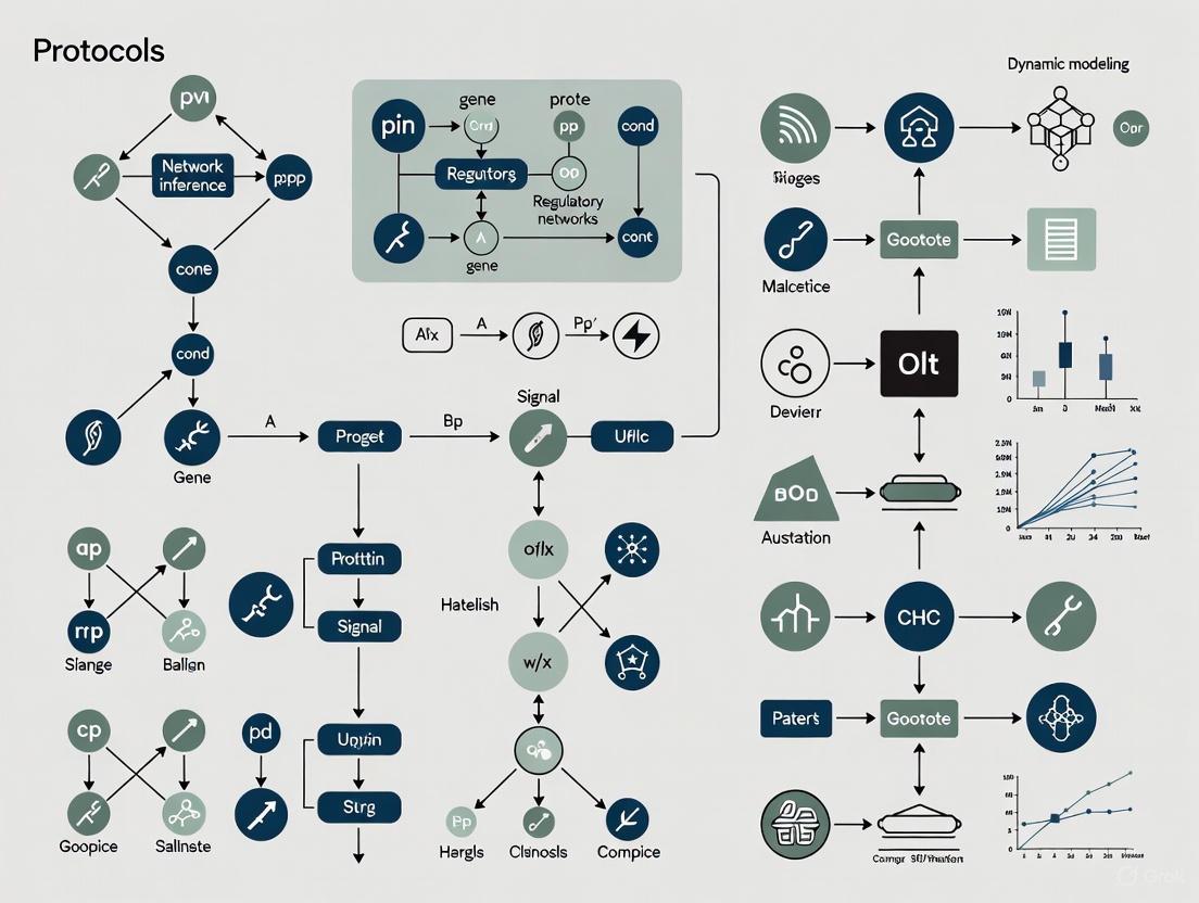
Network Inference and Dynamic Modeling in Systems Biology: A Comprehensive Protocol for Biomedical Research

Abstract

This article provides a comprehensive guide to network inference and dynamic modeling, essential for understanding complex biological systems in biomedical research and drug development. It covers foundational concepts, core methodologies for reconstructing gene regulatory and signaling networks, and protocols for dynamic model calibration using ordinary differential equations. The guide addresses critical challenges including parameter identifiability, model distinguishability, and optimization strategies. Furthermore, it details rigorous validation frameworks, credibility standards, and comparative analysis of model performance. By integrating these elements, this resource empowers researchers to build predictive, reliable computational models for advancing therapeutic discovery and personalized medicine.

Core Concepts and Problem Formulation in Biological Network Analysis

In systems biology, cellular processes are not governed by isolated entities but by complex, interconnected networks of molecular interactions. The network inference problem refers to the computational challenge of reconstructing these hidden regulatory architectures—where nodes represent biological molecules (e.g., genes, proteins, metabolites) and directed edges signify causal influences or regulatory relationships—from experimental observation data [1]. Solving this problem is foundational for understanding the underlying mechanisms of health and disease, enabling the identification of novel drug targets and the development of personalized therapeutic strategies.

The core challenge lies in the fact that biological networks are not directly observable; they must be deduced from often noisy, high-dimensional data like transcriptomics and metabolomics. This process is further complicated by the timescale separation across different molecular layers; for instance, metabolic changes can occur in minutes, while transcriptional responses unfold over hours [1]. This document outlines the formal definition of the network inference problem, presents core quantitative concepts, details standard and emerging experimental and computational protocols, and provides guidelines for the effective visualization of inferred networks.

Quantitative Foundations: Data Types and Distribution Summaries

The first step in network inference is to summarize and understand the raw, quantitative data, which typically consists of measurements of molecular abundance (e.g., gene expression, metabolite concentration) across different conditions or time points [2]. Except for very small amounts of data, understanding is difficult without a summary, which involves characterizing the distribution of the data—what values are present and how often they appear [2].

Table 1: Common Data Summarization Techniques for Quantitative Biological Data

Data Type	Summary Table Type	Key Statistics	Visualization Methods	Example in Biology
Continuous (e.g., metabolite concentration)	Frequency Table with Bins [2]	Counts, Percentages [2]	Histogram [2]	Distribution of birth weights in a population [2]
Discrete Quantitative (e.g., gene copy number)	Frequency Table [2]	Counts, Percentages [2]	Histogram, Bar Chart [2]	Number of severe cyclones per year [2]
Categorical / Survey (e.g., patient stratification)	Frequency Table, Grid [3]	Percentages, Row Percentages [3]	Bar Chart, Pie Chart	Likelihood of product purchase survey data [3]
Numeric Grid (e.g., brand consumption)	Summary Table of Variable Sets [3]	Averages, Medians, Percentages [3]	Heat Map, Table	Weekly consumption of different cola brands [3]

For continuous data, creating a frequency table requires grouping data into exhaustive and mutually exclusive intervals, or 'bins'. Care must be taken to define bin boundaries with more decimal places than the recorded data to avoid ambiguity regarding which bin an observation belongs to [2]. A histogram is a graphical representation of this frequency table, where the width of a bar represents a bin and the height represents the frequency (count or percentage) of observations within that range [2]. The choice of bin size and boundaries can significantly impact the histogram's appearance and interpretation [2].

Experimental Protocols for Data Generation

High-quality data is a prerequisite for reliable network inference. The following protocols describe standard methodologies for generating key data types.

Protocol: Bulk Metabolomic Profiling via Mass Spectrometry

This protocol describes the acquisition of bulk metabolomic data, which captures the relative or absolute abundances of small molecules in a biological sample.

• 1. Sample Collection and Preparation: Snap-freeze tissue or quench cell culture in liquid nitrogen to instantly halt metabolic activity. Homogenize the sample in a pre-chilled methanol:water solvent mixture to extract metabolites. Remove debris by centrifugation.
• 2. Data Acquisition via Liquid Chromatography-Mass Spectrometry (LC-MS): Separate metabolites in the extract using a reverse-phase liquid chromatography (LC) column. Ionize the separated metabolites using electrospray ionization (ESI) and analyze them with a high-resolution mass spectrometer (MS). Acquire data in both positive and negative ionization modes for comprehensive coverage.
• 3. Data Pre-processing: Convert raw instrument data files to an open format (e.g., .mzML). Perform peak picking, alignment, and integration using software (e.g., XCMS, Progenesis QI) to generate a feature table. This table contains metabolite identities (or features) as rows, samples as columns, and peak intensities as values.
• 4. Data Normalization: Normalize the feature table to correct for technical variation. Common methods include normalization by total ion intensity, internal standards (e.g., stable isotope-labeled compounds), or probabilistic quotient normalization.

Protocol: Single-Cell RNA Sequencing (scRNA-seq) using 10X Genomics

This protocol details the generation of transcriptomic data at single-cell resolution, capturing cellular heterogeneity.

• 1. Single-Cell Suspension Preparation: Dissociate solid tissue or harvest cells to create a single-cell suspension. It is critical to maintain high cell viability (>90%) and prevent clumping. Filter the suspension through a flow cytometry-compatible strainer.
• 2. Cell Barcoding and Library Preparation using 10X Genomics Chromium: Load the cell suspension, barcoded gel beads, and partitioning oil onto a 10X Genomics Chromium chip. The system partitions thousands of individual cells into nanoliter-scale droplets, each containing a uniquely barcoded bead. Within each droplet, cell lysis and reverse transcription occur, labeling the mRNA from each cell with its unique barcode.
• 3. Library Construction and Sequencing: Break the emulsion, purify the barcoded cDNA, and prepare sequencing libraries following the manufacturer's instructions. This typically involves cDNA amplification, fragmentation, and the addition of adapters and sample indices. Pool libraries and sequence on an Illumina platform (e.g., NovaSeq) to a sufficient depth (e.g., 50,000 reads per cell).
• 4. scRNA-seq Data Pre-processing: Demultiplex the raw sequencing data using the cell barcodes and unique molecular identifiers (UMIs). Align reads to a reference genome (e.g., with STARsolo or Cell Ranger) and generate a gene expression matrix where rows are genes, columns are cell barcodes, and values are UMI counts. Perform quality control to remove empty droplets, doublets, and low-quality cells based on metrics like UMIs per cell and mitochondrial gene percentage.

Computational Protocols for Network Inference

Once quantitative data is generated and summarized, computational methods are applied to infer the network. Below are two protocols representing state-of-the-art approaches.

Protocol: Multi-omic Network Inference with MINIE

MINIE is a computational method that integrates bulk metabolomic and single-cell transcriptomic time-series data through a Bayesian regression framework, explicitly modeling the timescale separation between molecular layers [1].

• 1. Input Data Preparation: Format your data into two matrices:
  • Transcriptomic Data (Slow Layer): A matrix G of size (number of time points × number of cells × number of genes) from scRNA-seq.
  • Metabolomic Data (Fast Layer): A matrix M of size (number of time points × number of metabolites) from bulk metabolomics.
• 2. Model Formalization using Differential-Algebraic Equations (DAEs): Formalize the system dynamics using DAEs to handle timescale separation [1]: d(g)/dt = f(g, m, b_g; θ) + ρ(g, m)w (Differential eq. for slow transcriptomic dynamics) d(m)/dt = h(g, m, b_m; θ) ≈ 0 (Algebraic eq. for fast metabolic dynamics, assuming quasi-steady-state) Here, g is gene expression, m is metabolite concentration, b are baseline effects, θ are model parameters, and w is noise.
• 3. Transcriptome-Metabolome Mapping Inference: Use the algebraic constraint to linearize the fast metabolic dynamics [1]: 0 ≈ A_mg * g + A_mm * m + b_m m ≈ -A_mm⁻¹ * A_mg * g - A_mm⁻¹ * b_m Infer the interaction matrices A_mg (gene-metabolite) and A_mm (metabolite-metabolite) by solving a sparse regression problem, constrained by prior knowledge of human metabolic reactions [1].
• 4. Regulatory Network Inference via Bayesian Regression: Using the mapped data and the DAE framework, infer the final intra- and inter-layer regulatory network topology. The Bayesian approach provides robustness to noise and yields posterior probabilities for inferred edges, allowing researchers to rank interactions by confidence [1].

Protocol: GRN Inference from scRNA-seq with DAZZLE

DAZZLE addresses the prevalent "dropout" problem (false zero counts) in scRNA-seq data to improve Gene Regulatory Network (GRN) inference. It uses a novel Dropout Augmentation (DA) technique for model regularization [4].

• 1. Input Data Transformation: Start with a scRNA-seq gene expression count matrix X (cells × genes). Transform the data to reduce variance and avoid log(0) using log(X + 1).
• 2. Dropout Augmentation (Model Regularization): During each training iteration, randomly select a small proportion of the non-zero expression values and set them to zero. This artificially simulates additional dropout events, exposing the model to multiple noisy versions of the data and preventing it from overfitting to the specific dropout pattern in the original dataset [4].
• 3. Model Training with a Structured Autoencoder: Employ a variational autoencoder (VAE) architecture where the adjacency matrix A of the GRN is a parameter. The model is trained to reconstruct its input. A noise classifier is trained simultaneously to identify and down-weight values likely to be dropout noise during reconstruction [4].
• 4. Network Extraction and Sparsity Control: After training, the weights of the learned adjacency matrix A are retrieved as the inferred GRN. DAZZLE improves stability by delaying the application of sparsity-inducing loss terms and uses a closed-form prior, leading to faster computation and reduced model size compared to predecessors like DeepSEM [4].

Table 2: Key Research Reagent Solutions for Network Inference Studies

Reagent / Resource	Function	Example Use Case
10X Genomics Chromium	A microfluidic platform for partitioning single cells into droplets for barcoding and scRNA-seq library preparation [4].	Generating high-throughput single-cell transcriptomic data for input into GRN inference tools like DAZZLE or MINIE.
LC-MS/MS System	An analytical chemistry instrument that separates complex mixtures (LC) and identifies/quantifies components with high sensitivity and specificity (MS/MS).	Profiling metabolite abundances for bulk metabolomic data, a key input for multi-omic inference with MINIE [1].
Stable Isotope-Labeled Internal Standards	Chemically identical analogs to target metabolites with replaced atoms (e.g., ¹³C, ¹⁵N), used for absolute quantification in mass spectrometry.	Added to biological samples during metabolomic extraction to correct for losses during preparation and matrix effects during ionization.
Curated Metabolic Network (e.g., Recon3D)	A knowledgebase of manually curated human metabolic reactions, pathways, and metabolites [1].	Used as a prior to constrain the solution space for metabolite-metabolite and gene-metabolite interactions during inference with MINIE [1].
BEELINE Benchmarking Framework	A computational toolkit and standardized set of benchmarks for evaluating the performance of GRN inference algorithms [4].	Used to validate and compare the accuracy of new inference methods like DAZZLE against existing state-of-the-art tools.

Biological systems are governed by complex, interconnected networks that coordinate cellular functions, enabling organisms to grow, adapt, and respond to their environment. These networks—comprising transcriptional, signaling, metabolic, and protein-protein interactions—form the core framework of systems biology. The study of these networks through inference and dynamic modeling has become paramount for deciphering biological complexity, from fundamental cellular processes to disease mechanisms such as cancer. This article details the experimental and computational protocols essential for investigating the structure and dynamics of these biological networks, providing a practical guide for researchers and drug development professionals engaged in systems biology research.

Transcriptional Regulatory Networks (TRNs)

Transcriptional Regulatory Networks (TRNs) map the interactions between transcription factors and their target genes, revealing the program that controls gene expression. Inferring these networks from high-throughput data is crucial for understanding cell identity and fate decisions.

Key Methods and Protocols

Network Inference with Single-Cell Data: Accurately inferring GRNs from high-dimensional and noisy single-cell data remains a significant challenge. A robust hybrid framework, GGANO, integrates Gaussian Graphical Models for learning conditional independence between genes with Neural Ordinary Differential Equations for dynamic modeling and inference. This method demonstrates superior accuracy and stability compared to conventional approaches, particularly under high-noise conditions, and enables the inference of stochastic dynamics from single-cell data [5].

Independent Component Analysis (ICA) for TRN Expansion: A powerful approach for dissecting regulatory structures involves applying Independent Component Analysis (ICA) to large transcriptome compendia. This signal decomposition algorithm processes hundreds of RNA-seq datasets from diverse conditions and genetic backgrounds to identify "iModulons"—independently modulated gene sets. This method has been successfully used to map the TRN of Bacteroides thetaiotaomicron, a gut symbiont, leading to a significant expansion of its known regulatory network by establishing novel regulator-regulon relationships and functionally characterizing previously unknown transcription factors like specific ECF-σ factors [6].

Table 1: Core Methods for Transcriptional Network Inference

Method	Principle	Application Example	Key Advantage
GGANO	Hybrid of Gaussian Graphical Models & Neural ODEs	Inferring gene dynamics from single-cell RNA-seq data [5]	High accuracy and robustness to noise; models stochastic dynamics
Independent Component Analysis (ICA)	Signal decomposition to identify co-regulated gene sets	Mapping regulons and characterizing ECF-σ factors in B. thetaiotaomicron [6]	Systematically expands known TRNs from large transcriptome compendia
CRISPRi-mediated Repression	Targeted knockdown of regulators to observe network perturbation	Functional validation of regulator-regulon relationships [6]	Enables causal validation of inferred regulatory links

Experimental Workflow: TRN Reconstruction

The following diagram outlines a general workflow for reconstructing and validating a Transcriptional Regulatory Network, integrating computational inference and experimental validation.

Research Reagent Solutions for TRN Studies

Table 2: Essential Reagents for Transcriptional Network Analysis

Reagent / Tool	Function in Protocol
Anhydrotetracycline	Inducer for CRISPRi/dCas9 systems to control sgRNA expression [6].
Erythromycin & Gentamicin	Selection antibiotics for maintaining plasmids in bacterial systems [6].
BHIS Broth & Anaerobic Minimal Medium	Specialized culture media for maintaining and experimenting on fastidious microorganisms like B. thetaiotaomicron [6].
dCas9 Expression Vector	Engineered plasmid for targeted gene repression without cleavage in CRISPRi validation [6].
Single Guide RNA (sgRNA) Libraries	Designed RNAs to target dCas9 to specific genomic loci for repression [6].

Signaling Networks

Signaling networks transmit information from a cell's exterior to its interior, triggering appropriate cellular responses through complex cascades of molecular interactions. Detailed protocols are essential for dissecting this complexity.

Key Methods and Protocols

Comprehensive Protocol Resources: "Signal Transduction Protocols, 3rd Edition" provides a collection of experimental methods focused on receptor-ligand interactions and the intricacies of integrated signaling pathways. These protocols are designed to enhance critical thinking and knowledge retention in signal transduction research [7].

Specialized Laboratory Techniques: Research groups, such as the Cell Signal Transduction Networks Laboratory, develop and publish specific, peer-reviewed methodologies for studying signaling networks. These protocols offer detailed, reproducible steps for particular experimental contexts [8].

Experimental Workflow: Signaling Pathway Analysis

A generalized workflow for analyzing a signaling pathway is shown below, from stimulus to response measurement.

Metabolic Networks

Metabolic networks represent the complete set of biochemical reactions within a cell, determining its metabolic capabilities and resource utilization. Their modeling is critical for understanding diseases like cancer and for metabolic engineering in plants and microbes.

Key Methods and Protocols

Flux Balance Analysis (FBA): FBA is a constraint-based modeling approach used to predict the flow of metabolites (flux) through a genome-scale metabolic network at steady state. It is widely applied to model primary and specialized metabolism and to predict phenotypes resulting from genetic or environmental perturbations [9].

13C-Metabolic Flux Analysis (13C-MFA): This technique relies on feeding cells isotope-labeled substrates (e.g., 13C-glucose) and using mass spectrometry to track the incorporation of the label into intermediate metabolites. The resulting isotopic distribution data allows for the quantitative estimation of in vivo metabolic flux rates in central carbon metabolism [10] [9].

Seahorse Metabolic Flux Analysis: This platform provides a real-time, live-cell assay for measuring key parameters of mitochondrial function, specifically the oxygen consumption rate (OCR) and extracellular acidification rate (ECAR), which serve as proxies for oxidative phosphorylation and glycolysis, respectively. It is extensively used in cancer research to profile metabolic phenotypes [10].

Dynamic Metabolic Modeling: Also known as kinetic modeling, this approach uses differential equations to describe the temporal adjustments of metabolic systems. It is particularly valuable for modeling processes that are not at steady state, such as metabolic responses to environmental stimuli or during developmental transitions [9].

Experimental Workflow: Metabolic Flux Analysis

A standard workflow for 13C-Metabolic Flux Analysis is depicted below, showing the integration of wet-lab and computational steps.

Research Reagent Solutions for Metabolic Studies

Table 3: Essential Reagents for Metabolic Network Analysis

Reagent / Tool	Function in Protocol
13C-Labeled Substrates (e.g., 13C-Glucose)	Tracers for MFA to follow carbon fate through metabolic pathways [10] [9].
Seahorse XF Analyzer Kits	Pre-formulated assay kits to measure OCR and ECAR in live cells [10].
Genetically Encoded Biosensors	Fluorescent tools for real-time monitoring of metabolite levels (e.g., NADH, ATP) in live cells [10].
Anaerobic Chamber	Equipment for maintaining strict anaerobic conditions for culturing obligate anaerobes [6].

Protein-Protein Interaction (PPI) Networks

PPI networks map the physical associations between proteins, forming the backbone of most cellular machineries and signaling complexes.

Key Methods and Protocols

Mass Photometry: This technique measures the optical contrast generated by single protein complexes as they bind to a glass-water interface. It enables mass-resolved quantification of biomolecular mixtures, making it ideal for characterizing protein complexes, their stoichiometry, and stability without the need for labels [11].

Proximity-Dependent Labeling Techniques: Protocols such as BioID (proximity-dependent biotin identification) use engineered enzymes to biotinylate proteins in close proximity to a protein of interest. This allows for the mapping of protein interactomes in living cells, capturing weak or transient interactions that are difficult to detect with traditional methods.

Integrated Network Modeling in Systems Biology

Biological networks do not operate in isolation. A central goal of systems biology is to integrate these different network layers to build comprehensive models of cellular function.

Network Inference and Modeling Principles

Theoretical methods are indispensable for interpreting high-throughput biological data. A systems biology perspective emphasizes that methods for graph inference (reconstructing networks), graph analysis (mining networks for information), and dynamic network modeling (linking structure to behavior) are most powerful when they lead to testable biological predictions [12]. This integrated approach is applicable across model organisms, from human cells to plants [12].

Machine Learning and Future Perspectives

The field is rapidly advancing with the integration of machine learning (ML) technologies. In metabolic modeling, ML is being explored to predict enzyme kinetics, optimize metabolic models, and interpret complex multi-omics datasets [9]. Similarly, frameworks like GGANO that combine traditional models with neural networks represent the future of dynamic network inference from single-cell data [5]. These tools are poised to unravel the profound complexity and heterogeneity of biological systems.

Modern systems biology relies on high-throughput omics technologies to decipher the complex network architecture and dynamic behaviors of cellular systems. Single-cell RNA-sequencing (scRNA-seq) has revolutionized transcriptomic analysis by enabling researchers to investigate gene expression profiles at individual cell resolution, revealing cellular heterogeneity in complex biological systems that was previously obscured by bulk sequencing approaches [13]. The emergence of spatial biology and multi-omic integrations now provides unprecedented insights into how cells, molecules, and biological processes are organized and interact within their native tissue environments [14]. These technological advancements are fueling breakthroughs in oncology, neuroscience, immunology, and precision medicine by allowing researchers to study biological systems as integrated networks rather than collections of isolated components [12] [14].

The integration of scRNA-seq with other omics modalities creates a powerful framework for network inference and dynamic modeling in systems biology. Cells utilize intricate signaling and regulatory pathways connecting numerous constituents—including DNA, RNA, proteins, and small molecules—to coordinate multiple functions and adapt to changing environments [12]. High-throughput experimental methods now enable the simultaneous measurement of thousands of molecular interactions, generating complex datasets that require sophisticated theoretical approaches for meaningful interpretation [12]. This application note details standardized protocols and methodologies for leveraging these technologies to construct predictive models of cellular behavior, with particular emphasis on network inference, analysis, and modeling in systems biology research.

Single-Cell RNA-Sequencing: Core Principles and Workflows

Fundamental Technological Concepts

Single-cell RNA-sequencing represents a paradigm shift from bulk RNA-seq, with the key distinction being whether each sequencing library reflects an individual cell or a grouped cell population [13]. This technology has brought about a revolutionary change in the transcriptomic world by enabling comprehensive analysis of cellular heterogeneity, allowing researchers to observe how different cells behave at single-cell levels and providing new insights into biological processes [13]. The technique is particularly valuable for addressing crucial biological inquiries related to cell heterogeneity, early embryo development, and tumor diversity, especially in cases involving limited cell numbers [13].

The scRNA-seq workflow presents unique technical challenges distinct from bulk sequencing approaches, including scarce transcripts in single cells, inefficient mRNA capture, losses in reverse transcription, and bias in cDNA amplification due to the minute amounts of starting material [13]. scRNA-seq data are characterized by high dimensionality, noise, and sparsity, necessitating specialized computational tools for proper interpretation [15] [13]. During quality control, researchers must identify and remove low-quality individual cells and any data that might represent multiple cells (doublets), while being cautious about applying normalization techniques designed for bulk RNA-sequencing, as these can introduce significant errors into scRNA-seq data [13].

The following diagram illustrates the core steps in a standard scRNA-seq workflow, from sample preparation through data analysis:

Figure 1: scRNA-seq Workflow. The process begins with sample preparation and progresses through library preparation, sequencing, and computational analysis.

Comparative Analysis of scRNA-seq Methodologies

The table below provides a comprehensive comparison of major scRNA-seq protocols, highlighting their key technical specifications and applications:

Table 1: Comparison of Single-Cell RNA-Sequencing Protocols

Protocol	Isolation Strategy	Transcript Coverage	UMI	Amplification Method	Unique Features and Applications
Smart-Seq2	FACS	Full-length	No	PCR	Enhanced sensitivity for detecting low-abundance transcripts; generates full-length cDNA ideal for isoform analysis [13].
Drop-Seq	Droplet-based	3'-end	Yes	PCR	High-throughput and low cost per cell; scalable to thousands of cells simultaneously [16] [13].
inDrop	Droplet-based	3'-end	Yes	IVT	Uses hydrogel beads; low cost per cell; efficient barcode capture [13].
CEL-Seq2	FACS	3'-only	Yes	IVT	Linear amplification reduces bias compared to PCR methods [13].
Seq-Well	Droplet-based	3'-only	Yes	PCR	Portable, low-cost, easily implemented without complex equipment [13].
DroNC-Seq	Droplet-based	3'-only	Yes	PCR	Specialized for single-nucleus sequencing, minimal dissociation bias [16] [13].
SPLiT-Seq	Not required	3'-only	Yes	PCR	Combinatorial indexing without physical separation; highly scalable and low cost [13].
MATQ-Seq	Droplet-based	Full-length	Yes	PCR	Increased accuracy in quantifying transcripts; efficient detection of transcript variants [13].
Fluidigm C1	Droplet-based	Full-length	No	PCR	Microfluidics-based single-cell capture; precise cell handling [16] [13].

Cell Isolation Strategies

The initial stage of performing scRNA-seq involves extracting viable individual cells from the tissue of interest. The table below summarizes the primary methods for cell preparation and isolation:

Table 2: Cell Isolation Methods for scRNA-seq

Method	Principle	Advantages	Limitations	Applications
FACS	Fluorescent-activated cell sorting	High purity and specificity based on surface markers; can select rare cell populations	Requires specialized equipment; potential for cellular stress during sorting	Ideal for targeted isolation of specific cell types using antibody-based selection [13].
Droplet-based	Microfluidic encapsulation of cells	High-throughput processing of thousands of cells; cost-effective per cell	Limited control over individual cell selection; potential for multiple cells per droplet (doublets)	Excellent for unbiased profiling of complex tissues and tumor microenvironments [16] [13].
Combinatorial Indexing	Split-pooling with barcodes	Does not require physical separation; can process millions of cells; no specialized equipment needed	Complex barcode design and analysis; potential index hopping	Suitable for very large-scale studies with limited sample material [13].

Novel methodologies have emerged to address specific research challenges. For instance, single-nucleus RNA-seq (snRNA-seq) is employed when tissue dissociation is problematic or when working with frozen samples or fragile cells [13]. Split-pooling techniques using combinatorial indexing (cell barcodes) offer distinct advantages over isolation of intact single cells, including the ability to handle large sample sizes (up to millions of cells) and greater efficiency in parallel processing of multiple samples while eliminating the need for expensive microfluidic devices [13].

Advanced Multi-Omics Integration and Spatial Biology

Emerging Multi-Omic Technologies

The field of single-cell analysis has evolved beyond transcriptomics to include multi-omic approaches that simultaneously measure multiple molecular layers from the same cells. SUM-seq (single-cell ultra-high-throughput multiplexed sequencing) represents a recent advancement that enables cost-effective, scalable co-assaying of chromatin accessibility and gene expression in single nuclei [17]. This technology allows profiling of hundreds of samples at the million-cell scale, outperforming current high-throughput single-cell methods in both throughput and data quality [17].

SUM-seq builds on a two-step combinatorial indexing approach, extending it to multi-omic applications. The method involves several key steps: (1) nuclei isolation and fixation, (2) introduction of unique sample indices for both ATAC and RNA modalities, (3) pooling of samples, (4) microfluidic barcoding, and (5) modality-specific library preparation and sequencing [17]. Performance metrics of SUM-seq consistently demonstrate high quality for both snRNA (UMIs and genes per cell) and snATAC (fragments in peaks per cell, TSS enrichment score), with library complexity metrics outperforming other ultra-high-throughput assays [17].

Spatial Biology and Tissue Context

Spatial biology has emerged as a transformative discipline that enables researchers to study how cells, molecules, and biological processes are organized and interact within their native tissue environments [14]. By combining spatial transcriptomics, proteomics, metabolomics, and high-plex multi-omics integration with advanced imaging, spatial biology provides unprecedented insights into disease mechanisms, cellular interactions, and tissue architecture [14].

The global spatial biology market is experiencing rapid growth, projected to reach $6.39 billion by 2035, with a compound annual growth rate of 13.1% [14]. This expansion is driven by rising investments in spatial transcriptomics for precision medicine, the growing importance of functional protein profiling in drug development, and the expanding use of retrospective tissue analysis for biomarker research [14]. Leading players are shaping the competitive landscape through partnerships, acquisitions, and product innovations, with companies like Bruker Corporation, Vizgen, Akoya Biosciences, and 10x Genomics advancing integrated spatial solutions [14].

Research Reagent Solutions for Multi-Omic Studies

Table 3: Essential Research Reagents and Platforms for scRNA-seq and Multi-Omics

Reagent/Platform	Function	Application Notes
10x Chromium	Microfluidic platform for single-cell partitioning	Enables high-throughput cell barcoding and library preparation; widely adopted for droplet-based scRNA-seq and multi-ome applications [17].
Tn5 Transposase	Tagmentase for chromatin accessibility profiling	Loaded with barcoded oligos in SUM-seq for indexing accessible genomic regions in ATAC sequencing [17].
Barcoded Oligo-dT Primers	Cell barcoding during reverse transcription	Critical for introducing unique cell identifiers during cDNA synthesis; enables sample multiplexing [17].
Polyethylene Glycol (PEG)	Reverse transcription enhancer	Increases number of UMIs and genes detected per cell (~2.5- and ~2-fold respectively) with minor impact on ATAC quality [17].
Glyoxal Fixative	Nuclear fixation and preservation	Maintains sample integrity for asynchronous sampling; compatible with cryopreservation for prolonged storage [17].
Blocking Oligonucleotides	Reduces barcode hopping	Minimizes index cross-contamination in overloaded droplets, particularly important for ATAC modality [17].
Unique Molecular Identifiers (UMIs)	Correction for PCR amplification bias	Molecular tags that distinguish original RNA molecules from PCR duplicates; essential for accurate transcript quantification [13].

Network Inference and Dynamic Modeling from Single-Cell Data

Computational Framework for Network Inference

The complexity and high-dimensional nature of single-cell data necessitate advanced computational approaches for network inference and dynamic modeling. GGANO represents a recent hybrid framework that integrates Gaussian Graphical Models for conditional independence learning with Neural Ordinary Differential Equations for dynamic modeling and inference [5]. Benchmark analyses demonstrate that GGANO achieves superior accuracy and stability compared to existing methods, particularly under high-noise conditions commonly encountered in scRNA-seq data [5].

Gene regulatory networks (GRNs) form the foundation of cellular decision-making processes, and accurately inferring GRN architecture from high-dimensional and noisy single-cell data remains a major challenge in systems biology [5]. Conventional approaches often struggle with robustness and interpretability, particularly when applied to complex biological processes such as cell fate decisions and complex diseases [5]. The application of GGANO to epithelial-mesenchymal transition (EMT) datasets has enabled researchers to uncover intermediate cellular states and identify key regulatory genes driving EMT progression [5].

Bayesian Multimodel Inference for Enhanced Certainty

Mathematical models are indispensable for studying the architecture and behavior of intracellular signaling networks, but it is common to develop multiple models to represent the same pathway due to phenomenological approximations necessitated by incomplete observation of intermediate steps in intracellular signaling pathways [18]. Bayesian multimodel inference (MMI) has emerged as a powerful approach to increase certainty in systems biology predictions when leveraging a set of potentially incomplete models [18].

The Bayesian MMI workflow involves: (1) calibrating available models to training data by estimating unknown parameters with Bayesian inference, (2) combining the resulting predictive probability densities using MMI, and (3) generating improved multimodel predictions of important quantities in systems biology studies [18]. This approach constructs predictors by taking a linear combination of predictive densities from each model: p(q|dtrain, 𝔐K) = Σ{k=1}^K wk p(qk|Mk, dtrain), with weights wk ≥ 0 that sum to 1 [18]. Application of MMI to ERK signaling pathway models has demonstrated increased certainty in predictions and robustness to changes in model composition and data uncertainty [18].

Network Inference Workflow

The following diagram illustrates the integrated computational pipeline for inferring gene regulatory networks from single-cell multi-omics data:

Figure 2: Network Inference Pipeline. Computational workflow for reconstructing gene network structure and dynamics from single-cell data.

Applications in Drug Discovery and Development

Model-Informed Drug Development (MIDD)

The integration of high-throughput single-cell technologies with Model-Informed Drug Development (MIDD) represents a paradigm shift in pharmaceutical research and development. MIDD provides an essential framework for advancing drug development and supporting regulatory decision-making by offering quantitative predictions and data-driven insights that accelerate hypothesis testing, improve candidate assessment efficiency, and reduce costly late-stage failures [19].

The "fit-for-purpose" strategic roadmap for MIDD aligns modeling tools with key questions of interest (QOI), context of use (COU), and model impact across all stages of drug development—from early discovery to post-market lifecycle management [19]. This approach demonstrates how MIDD tools can enhance target identification, assist with lead compound optimization, improve preclinical prediction accuracy, facilitate First-in-Human (FIH) studies, optimize clinical trial design including dosage optimization, describe clinical population pharmacokinetics/exposure-response (PPK/ER) characteristics, and support label updates during post-approval stages [19].

Omics-Enhanced Large Language Models in Drug Discovery

Large language models (LLMs), originally developed for natural language processing, are emerging as powerful tools to address challenges in omics data analysis, including high dimensionality, noise, and heterogeneity [15]. These models capture complex patterns and infer missing information from large, noisy datasets, enabling new applications in drug discovery [15].

A three-part framework for leveraging omics-based LLMs includes: (1) analyzing how LLM architectures and learning paradigms handle challenges specific to genomics, transcriptomics, and proteomics data; (2) detailing LLM applications in key areas such as uncovering disease mechanisms, identifying drug targets, predicting drug response, and simulating cellular behavior; and (3) discussing how insights from omics-integrated LLMs can inform the development of drugs targeting specific pathways, moving beyond single targets toward strategies grounded in underlying disease biology [15]. This framework provides both conceptual insights and practical guidance for leveraging LLMs in omics-driven drug discovery and development [15].

Applications in Personalized Medicine and Therapeutic Innovation

Single-cell and spatial omics technologies are driving innovations in personalized medicine by enabling detailed characterization of disease mechanisms at cellular resolution. These approaches are particularly valuable in oncology, where they facilitate the identification of novel therapeutic targets through comprehensive analysis of tumor microenvironments, cellular heterogeneity, and drug resistance mechanisms [13] [20].

The application of these technologies extends to neuroscience, immunology, and rare diseases, where they contribute to biomarker discovery, patient stratification, and understanding of disease pathogenesis [14] [20]. The continued advancement and integration of single-cell multi-omics technologies with computational modeling approaches promise to transform therapeutic development and precision medicine over the coming decade [14] [19].

In systems biology, complex molecular interactions are abstracted into networks to facilitate computational analysis and hypothesis generation. A network or graph provides a mathematical framework comprising nodes (vertices representing biological entities like genes or proteins) and edges (connections representing interactions or relationships) [21] [22]. The choice of network representation—directed or undirected, signed or unsigned—is a fundamental methodological decision that directly influences the biological insights that can be derived from network inference and dynamic modeling protocols [22] [23]. Directed networks incorporate asymmetric relationships where edges originate from one entity and terminate at another, whereas undirected networks represent symmetric, reciprocal relationships [24] [22]. Similarly, signed networks label edges with positive (activation) or negative (inhibition) signs, while unsigned networks only indicate the presence or absence of an interaction without specifying its nature [25] [23]. This application note provides a structured comparison of these representations and detailed protocols for their application in systems biology research, with a specific focus on gene regulatory network (GRN) inference.

Theoretical Foundations and Comparative Analysis

Directed vs. Undirected Networks

Table 1: Fundamental Differences Between Directed and Undirected Networks

Feature	Directed Networks	Undirected Networks
Relationship Symmetry	Asymmetric (A→B does not imply B→A)	Symmetric (A-B implies B-A) [22]
Edge Representation	Arrows indicating direction [22]	Simple lines without direction [22]
Mathematical Formalization	Set of ordered pairs (E ⊆ V×V) [24]	Set of unordered pairs [22]
Connectivity	Path from A to B does not guarantee path from B to A [22]	Connectivity is always mutual
Centrality Measures	Separate in-degree and out-degree centrality [24]	Single degree centrality [22]
Typical Applications	Signal transduction, regulatory networks, web graphs, citation networks [24] [22]	Protein-protein interaction, co-expression networks, friendship networks [22] [23]

Directed networks, or digraphs, are characterized by edges with a specific orientation, where a connection from node A to node B (an arc) does not imply a reciprocal connection from B to A [24]. This directionality introduces asymmetry, meaning the adjacency matrix representing the network is typically not symmetric [24]. Key concepts in directed networks include in-degree (number of incoming edges) and out-degree (number of outgoing edges), which quantify a node's prominence as a receiver or source of influence, respectively [24]. Connectivity is assessed through strongly connected components (where every node is reachable from every other via directed paths) and weakly connected components (where connectivity holds only when ignoring edge directions) [24]. In contrast, undirected networks represent bidirectional relationships where a connection between node A and node B is inherently mutual [22]. The adjacency matrix for an undirected network is symmetric, and a single degree centrality measure suffices for each node [22]. The choice between these models should be guided by the nature of the biological relationships under investigation, the specific research questions, and the available data [22].

Signed vs. Unsigned Networks

Table 2: Comparison of Signed and Unsigned Network Representations

Feature	Signed Networks	Unsigned Networks
Edge Information	Includes sign (+ for activation, - for inhibition) [23]	Presence or absence of interaction only [23]
Biological Specificity	High; indicates nature of regulatory effect [23]	Low; indicates interaction without mechanistic detail
Correlation Treatment	Strong negative correlations may be treated as no connection [25]	Strong correlations (positive or negative) indicate connection [25]
Inference Complexity	Higher; requires determining sign of interaction	Lower; focus is on interaction existence
Analytical Utility	Essential for drawing biological insights on regulation [23]	Sufficient for theoretical work on network structure [23]
Recommended Use	Default for most biological applications [25]	When interaction type is unknown or irrelevant

Signed networks encode the nature of interactions, crucially distinguishing between activation (positive edges) and inhibition/repression (negative edges) [23]. This representation is vital for understanding the dynamic behavior of biological systems, as it allows modelers to distinguish between reinforcing and antagonistic relationships. The Causal Attitude Network (CAN) model is an example that conceptualizes attitudes as networks of causally interacting evaluative reactions, a framework that can be adapted for biological signaling networks [21]. In a signed network, the sign of a correlation matters; some methodologies suggest that strongly negatively correlated nodes should be considered unconnected, leading to a "signed" network where the adjacency matrix contains only non-negative values despite the sign information [25]. Unsigned networks, conversely, only represent whether an interaction exists, treating strong correlations—whether positive or negative—as connections [25] [23]. While unsigned networks are simpler to construct and are often used in theoretical work, signed networks are generally preferable for biological applications because they preserve critical information about the direction of regulatory effects, which is essential for functional insights and predictive modeling [25] [23].

Experimental Protocols for Network Inference

Protocol 1: Inferring a Signed, Directed Gene Regulatory Network from Single-Cell RNA-Seq Data

This protocol details the steps for reconstructing a gene regulatory network (GRN) from single-cell RNA-sequencing data, resulting in a directed and signed network that captures causal regulatory relationships and their activating/inhibitory nature.

1. Experimental Design and Data Generation

• Single-Cell RNA-Sequencing: Perform single-cell RNA-seq on a population of cells under the biological condition of interest (e.g., a disease state, developmental time point, or after a perturbation). Each cell provides a snapshot of the expression levels of all genes, resulting in a matrix where rows represent cells and columns represent genes [23] [26].
• Pseudo-Temporal Ordering: If the data is from a static, heterogeneous population (e.g., cells at different stages of a process), use computational tools (e.g., Monocle, PAGA) to infer a pseudo-temporal ordering of the cells. This creates a trajectory that mimics the dynamic process being studied [23].
• Gene Selection: Identify a subset of genes with high biological variance for network analysis. This is typically done by plotting the Coefficient of Variation (CV; standard deviation/mean) against the mean expression for all genes and selecting genes with significantly higher CVs than expected for their expression level [23].

2. Data Preprocessing and Normalization

• Quality Control: Filter out low-quality cells and genes with low expression.
• Normalization: Normalize the expression counts to account for technical variations (e.g., sequencing depth). Common methods include log-transformation or more sophisticated approaches designed for single-cell data [26].
• Input Data Structure: The final preprocessed data for N selected genes is represented as a set of random variables {X₁, X₂, ..., Xₙ}, where each variable corresponds to the expression level of a gene (a node in the future GRN) [23].

3. Network Inference Using a Regression-Based Algorithm

• Algorithm Selection: Choose a regression-based inference algorithm capable of producing directed and signed networks, such as GENIE3 or TIGRESS [23]. The core principle is to solve, for each gene j, a regression problem where the expression of j is predicted from the expression of all other genes i (where i ≠ j).
• Model Execution: For each target gene Xⱼ, the algorithm solves an equation of the form: Xⱼ = f(X₁, X₂, ..., Xₙ), excluding Xⱼ itself. The function f can be a tree-based model (as in GENIE3) or a linear regression model with feature selection. The weight of the edge Xᵢ → Xⱼ is derived from the importance of Xᵢ in predicting Xⱼ [23].
• Sign Assignment: Once the set of significant interactions (edges) is identified, determine the sign of each edge. This is typically achieved by calculating the correlation (e.g., Pearson or Spearman) between the expression levels of the regulator gene Xᵢ and the target gene Xⱼ across the single-cell data. A positive correlation yields a "+" sign (activation), and a negative correlation yields a "-" sign (inhibition) [23].

4. Output and Validation

• Network Output: The final output is a set of weighted, directed, and signed edge predictions. The weight represents the confidence that a real regulatory interaction exists, the direction indicates the inferred causal relationship (Xᵢ → Xⱼ), and the sign indicates the type of regulation [23].
• Validation: Evaluate the accuracy of the inferred network against a "gold standard" dataset if available (e.g., from DREAM Challenges) using precision-recall (PR) curves or receiver operating characteristic (ROC) curves. PR curves are often considered superior for this task [23]. Experimental validation, such as siRNA knockdown or CRISPR inhibition of predicted regulator genes followed by qPCR of target genes, is the ultimate confirmation.

Protocol 2: Constructing an Unsigned, Undirected Co-Expression Network

This protocol outlines the creation of a gene co-expression network, which is typically undirected and unsigned, used to identify groups of functionally related genes without inferring causality.

1. Data Input and Preprocessing

• Use a gene expression matrix from either bulk RNA-seq or single-cell RNA-seq data. Preprocess and normalize the data as described in Protocol 1, Step 2 [23].

2. Correlation Matrix Calculation

• Compute the pairwise correlation matrix for all selected genes. The Pearson correlation coefficient is commonly used, but other measures like Spearman rank correlation can be more robust to outliers [23].
• For each pair of genes (i, j), the correlation coefficient rᵢⱼ is calculated, resulting in a symmetric matrix.

3. Network Construction and Thresholding

• The correlation matrix itself represents a fully connected, weighted, undirected network. To obtain a biologically meaningful and sparse network, apply a threshold.
• Threshold Selection: Choose a correlation threshold (e.g., |r| > 0.7) or use a method like Weighted Gene Co-expression Network Analysis (WGCNA) to transform the correlation matrix into an adjacency matrix [23]. In WGCNA, a signed or unsigned adjacency matrix can be created using a power function (soft thresholding) to emphasize strong correlations.
• Adjacency Matrix: The final adjacency matrix A is defined such that Aᵢⱼ = |rᵢⱼ|^β for an unsigned network (or other transformations for signed), where β is the soft-thresholding power. This step reduces the impact of weak correlations [23].

4. Module Detection and Analysis

• Use the resulting adjacency matrix to detect modules (clusters) of highly interconnected genes. This is typically done with hierarchical clustering and dynamic tree cutting.
• The resulting network is undirected (edges represent mutual co-expression) and unsigned (edges do not distinguish between positive and negative co-regulation, though the underlying correlations do) [23]. The primary output is a set of gene modules for functional enrichment analysis.

The Scientist's Toolkit: Essential Reagents and Computational Tools

Table 3: Key Research Reagent Solutions for Network Inference and Validation

Item Name	Type	Function in Protocol
Single-Cell RNA-Seq Kit (e.g., 10x Genomics)	Wet-lab Reagent	Generates the primary gene expression matrix from individual cells, the foundational data for network inference [23] [26].
DREAM Challenge Datasets	Computational Resource	Provide gold standard benchmarks with known network structures for objective algorithm evaluation and validation [23].
GENIE3 / TIGRESS	Software Algorithm	Regression-based methods for inferring directed GRNs from expression data [23].
WGCNA R Package	Software Algorithm	Constructs undirected co-expression networks and identifies functional gene modules from correlation matrices [23].
siRNA or CRISPR-Cas9 Kit	Wet-lab Reagent	Enables experimental perturbation (knockdown/knockout) of predicted regulator genes to validate inferred edges in the network [23].

Advanced Topics: Dynamic and Multi-Scale Network Modeling

Biological systems are inherently dynamic. Moving beyond static network snapshots to model temporal dynamics is a key frontier. The ProbRules approach combines probabilities and logical rules to represent system dynamics across multiple scales, which is particularly useful for signal transduction networks where reactions occur in different spatial and temporal frames [27]. In this framework, the state of an interaction is represented by a probability, and a set of rules drives the evolution of these probabilities over time, allowing the model to capture the logic of succession in interaction activities [27].

For inferring dynamic networks from single-cell data, methods like GRIT (Gene Regulation Inference by Transport) have been introduced. GRIT uses optimal transport theory to fit a differential equation model to data by tracking the evolution of the cell distribution over time, effectively inferring the underlying GRN [26]. Furthermore, statistical formulations that connect single-cell stochastic dynamics to network inference on population-averaged data are crucial for proper experimental design and interpretation [28]. These models start from a description of stochastic dynamics in single cells and, through a series of assumptions, arrive at a general statistical framework for network inference from discretely observed data [28].

Network motifs are statistically over-represented, recurring patterns of interconnections found in complex biological networks [29] [30]. These small subgraphs function as fundamental computational circuits that define the dynamic behavior and functional capabilities of cellular regulatory systems [23] [31]. As building blocks of complex networks, motifs perform specific information-processing functions including signal amplification, noise filtering, temporal regulation, and response acceleration [32] [29]. The identification and characterization of these motifs provide crucial insights into the design principles of biological systems and enable the development of predictive dynamic models.

In transcriptional regulatory networks, three-node motifs are particularly significant for their well-characterized dynamical properties. Among the thirteen possible three-node directed subgraphs, only a select few are found to be statistically overrepresented in natural networks, suggesting they have been evolutionarily selected for their functional advantages [30] [33]. The most extensively studied of these include feed-forward loops, cascades, and fan-ins/outs, each conferring distinct information-processing capabilities to the network [23] [29]. This application note provides a comprehensive overview of these common network motifs, detailing their structures, dynamical functions, and experimental protocols for their inference and analysis within systems biology research.

Feed-Forward Loops: Structure, Dynamics, and Experimental Analysis

Architectural Configurations and Functional Classification

The feed-forward loop (FFL) is one of the most prevalent and well-characterized network motifs in biological systems, consistently identified as statistically overrepresented in transcriptional networks from E. coli to humans [32] [33]. This three-node pattern consists of a top regulator (X) that controls a target gene (Z) both directly and indirectly through a second regulator (Y), forming two parallel regulatory paths [32]. The FFL motif exists in eight possible configurations depending on the activation/repression nature of each interaction, which are broadly categorized as coherent or incoherent [32] [33].

In coherent FFLs (C-FFLs), the direct regulatory path from X to Z and the indirect path through Y have the same overall sign, resulting in reinforcing regulation. Conversely, in incoherent FFLs (I-FFLs), the direct and indirect paths have opposing signs, creating potentially opposing regulatory effects [32]. Among these configurations, the coherent type 1 (C1-FFL, with all three interactions being activations) and incoherent type 1 (I1-FFL, where X activates both Y and Z, but Y represses Z) occur with the highest frequency in natural networks [32]. The abundance of these specific configurations reflects their particular functional utility in cellular information processing.

Figure 1: Basic structure of a coherent type-1 feed-forward loop (C1-FFL) with all activating interactions. Node X regulates Z both directly and through regulator Y.

Dynamical Properties and Biological Functions

The specific temporal dynamics and functional capabilities of FFLs depend on both their configuration (coherent/incoherent) and the logical rules (AND/OR) governing integration of signals at the Z promoter [32] [33]. The table below summarizes the key dynamical functions of major FFL types:

Table 1: Functional properties of common FFL configurations

FFL Type	Logic	Key Dynamical Function	Biological Examples
C1-FFL	AND	Sign-sensitive delay; Pulse filtering	Arabinose catabolism system in E. coli [33]
C1-FFL	OR	Off-delay; Response persistence	Not specified in sources
I1-FFL	AND	Pulse generation; Response acceleration	Galactose utilization system [32]
I1-FFL	OR	Accelerated shutdown	Not specified in sources

The C1-FFL with AND logic functions as a sign-sensitive delay element that filters out transient input signals [32] [33]. When the input signal appears, the motif introduces a delay in Z activation because both X and Y must be present to activate Z (AND logic). However, when the input signal disappears, Z expression shuts off immediately without delay. This asymmetric temporal response allows the system to distinguish between persistent and transient input signals, potentially filtering out stochastic noise in the cellular environment [32].

The I1-FFL with AND logic operates as a pulse generator and response accelerator [32]. When the input signal appears, X rapidly activates Z directly, leading to immediate expression. As Y accumulates, it begins to repress Z, resulting in a pulse-like expression pattern. This configuration can accelerate response times compared to simple regulation by generating a rapid initial burst of expression before settling into steady-state levels [32]. The functional versatility of FFLs explains their evolutionary conservation across diverse biological systems and their implementation in synthetic biology applications [32].

Experimental Protocol: Inference and Validation of FFLs

Objective: Identify and validate functional feed-forward loop motifs from gene expression data.

Materials and Reagents:

• Single-cell RNA sequencing data (scRNA-seq)
• Gene expression matrix (cells × genes)
• Computational resources for network inference
• Validation reagents (qPCR, CRISPRi, reporter constructs)

Procedure:

• Data Preprocessing

  • Filter genes based on coefficient of variation (CV) to select genes with high biological variance [23]
  • Normalize expression data using standard scRNA-seq pipelines
  • Address dropout events characteristic of scRNA-seq data [34]

• Network Inference

  • Apply multiple inference algorithms (e.g., PIDC, GENIE3, PHIXER) to generate candidate networks [23]
  • Extract all three-node subgraphs from the inferred network
  • Calculate statistical significance using Z-score comparison to randomized networks [33]: [ Z = \frac{N{\text{obs}} - \langle N{\text{rand}} \rangle}{\sigma{\text{rand}}} ] where (N{\text{obs}}) is the count in the observed network, (\langle N{\text{rand}} \rangle) is the mean count in randomized networks, and (\sigma{\text{rand}}) is the standard deviation.

• Motif Validation

  • Select top candidate FFLs for experimental validation
  • For each FFL (X→Y, X→Z, Y→Z), verify regulatory relationships using:
    • Chromatin Immunoprecipitation (ChIP) for transcription factor binding
    • CRISPRi-based repression of X and Y with measurement of Z expression
    • Reporter gene constructs with mutated binding sites
  • Test dynamic response to X induction/repression using time-course qPCR

• Functional Characterization

  • Measure temporal expression patterns of Z in response to X activation
  • Compare response dynamics to theoretical predictions
  • Assess noise-filtering capabilities under stochastic stimulation

Troubleshooting:

• High false-positive rates in network inference may require integration of prior knowledge [34]
• Biological variability may necessitate increased replicate numbers
• Confirming direct versus indirect regulation requires additional experimental approaches

Cascades and Fan-In/Fan-Out Motifs

Structural Properties and Network Context

Beyond FFLs, cascades and fan-in/fan-out motifs represent fundamental architectural patterns in regulatory networks. While these motifs may not always be statistically overrepresented in isolation, they form essential connective structures that contribute significantly to network dynamics [23].

Cascades (also referred to as regulatory paths) represent linear sequences of regulatory interactions where X regulates Y, which in turn regulates Z, creating a directional flow of information through the network [23]. Correlation-based network inference algorithms have been noted to demonstrate increased false positive rates for cascade structures, often misinterpreting them as direct regulations [23].

Fan-in motifs occur when multiple regulators converge on a single target gene, enabling integrative signal processing and combinatorial control [23] [29]. In contrast, fan-out motifs feature a single regulator controlling multiple target genes, facilitating coordinated expression of functionally related genes [23] [29].

Figure 2: Structural representations of cascade, fan-in, and fan-out network motifs.

Functional Significance in Regulatory Networks

The table below summarizes the key functional roles of these motifs and their detection by different inference algorithms:

Table 2: Functional properties of cascade, fan-in, and fan-out motifs

Motif Type	Functional Role	Algorithm Detection Performance
Cascade	Information transmission; Temporal delay	Increased false positives with correlation methods [23]
Fan-in	Combinatorial control; Signal integration	Regression methods perform poorly [23]
Fan-out	Coordinated expression; Single-input modules	Regression methods perform poorly [23]

Fan-in architectures allow for complex logical integration of multiple signals at promoter regions, enabling precise control of gene expression based on specific combinations of input signals [29]. This combinatorial control is essential for context-specific gene regulation in response to multiple environmental or developmental cues.

Fan-out structures, often organized as single-input modules (SIMs), enable synchronized expression of genes encoding functionally related proteins, such as enzymes in a metabolic pathway or components of a macromolecular complex [29]. This coordinated control ensures proper stoichiometry of interacting components and efficient resource allocation.

Regression-based network inference methods generally perform poorly in detecting both fan-in and fan-out motifs [23], highlighting the importance of employing multiple algorithmic approaches for comprehensive network mapping. Correlation-based methods, while generally simplistic, tend to perform relatively well on detecting feed-forward loops, fan-ins, and fan-outs, though with increased false positive rates for cascades [23].

Integrated Analysis of Network Motifs

Motif Aggregation and Higher-Order Organization

Network motifs do not function in isolation but rather aggregate to form higher-order structures that define the overall system behavior [35]. The specific ways in which motifs connect and cluster within networks reveal architectural principles that are characteristic of different biological systems [35]. Methods to quantify motif clustering (M~c~) have been developed to capture the propensity of motifs to share nodes, with different network types exhibiting distinctive clustering patterns [35].

In metabolic networks, type 6 FFL clusters (characterized by a single node that serves as input to all other nodes in the cluster) dominate, representing over 70% of FFL clustering in both E. coli and A. fulgidus metabolism [35]. This architecture reflects the broad use of common metabolites (such as ATP and ADP) by multiple biosynthetic pathways, creating highly interconnected functional modules [35].

The analysis of motif aggregation patterns provides insights into evolutionary constraints and functional requirements that shape network architecture. Different types of FFL clusters predominate in different network types, suggesting that specific clustering patterns are better suited to particular biological functions [35].

Advanced Protocol: Multi-Omic Network Inference with MINIE

Objective: Infer regulatory networks integrating transcriptomic and metabolomic data to capture cross-layer motif organization.

Materials and Reagents:

• Time-series scRNA-seq data
• Time-series bulk metabolomics data
• MINIE software package [1]
• Prior knowledge database of molecular interactions

Procedure:

• Data Preparation

  • Collect synchronized time-series transcriptomic and metabolomic data
  • Align temporal measurements from both omic layers
  • Normalize datasets using platform-specific methods

• Model Configuration

  • Implement Differential-Algebraic Equation (DAE) framework: [ \begin{array}{ll} \dot{g} = f(g,m,bg;\theta) + \rho(g,m)w \ \dot{m} = h(g,m,bm;\theta) \approx 0 \end{array} ] where (g) represents gene expression levels, (m) represents metabolite concentrations, and (\dot{m} \approx 0) reflects the timescale separation assumption [1].
  • Incorporate prior knowledge of metabolic reactions to constrain possible interactions

• Network Inference

  • Perform transcriptome-metabolome mapping using sparse regression
  • Infer intra-layer and cross-layer regulatory interactions via Bayesian regression
  • Generate consensus network integrating multiple inference runs

• Motif Analysis

  • Extract all three-node subgraphs from the inferred multi-omic network
  • Calculate statistical significance against appropriate null models
  • Identify statistically overrepresented motifs using z-score analysis
  • Characterize motif clustering patterns and inter-motif connections

• Experimental Validation

  • Select key cross-layer motifs for targeted validation
  • Use genetic perturbations (knockdown/overexpression) of transcriptomic nodes
  • Measure effects on metabolite levels via targeted mass spectrometry
  • Verify regulatory relationships using reporter assays

Applications:

• Identification of functional motifs that span molecular layers
• Discovery of metabolite-mediated regulatory pathways
• Characterization of multi-layer network architecture in disease states

Research Reagents and Computational Tools

Table 3: Essential research reagents and computational tools for network motif analysis

Resource Type	Specific Examples	Function/Application
Network Inference Algorithms	PIDC [23], GENIE3 [23] [34], PHIXER [23]	Inference of regulatory networks from expression data
Motif Discovery Tools	FANMOD [30], Kavosh [30], G-tries [30]	Identification of overrepresented network motifs
Statistical Frameworks	Exponential Random Graph Models (ERGMs) [31]	Assessment of motif significance controlling for network topology
Experimental Validation	CRISPRi, ChIP-seq, Reporter constructs	Verification of predicted regulatory interactions
Data Types	scRNA-seq [34], Bulk metabolomics [1]	Multi-omic measurements for network inference

Network motifs represent fundamental building blocks of biological systems, encoding specific information-processing functions that define cellular regulatory dynamics. The feed-forward loop, with its diverse configurations and functional capabilities, serves as a paradigm for understanding how simple regulatory architectures can generate complex temporal dynamics. Cascades and fan-in/fan-out motifs provide essential connective structures that enable information flow and signal integration throughout regulatory networks.

Advanced network inference methods, particularly those integrating multi-omic data and accounting for timescale separation between molecular layers, provide powerful approaches for identifying these motifs in biological systems [1]. The experimental protocols outlined here offer comprehensive frameworks for inferring, validating, and characterizing network motifs, enabling researchers to move from computational predictions to biological insights.

As systems biology continues to evolve, the analysis of motif organization and their higher-order aggregation will remain essential for understanding the design principles of biological systems and for engineering synthetic circuits with predictable functions. The integration of sophisticated computational approaches with rigorous experimental validation provides a pathway toward deciphering the regulatory logic that underpins cellular behavior.

Core Algorithms and Dynamic Model Construction for Network Inference

In the broader context of protocols for network inference and dynamic modeling in systems biology, the reconstruction of interaction graphs from experimental data is a fundamental task [36]. Gene co-expression networks are a powerful representation for this purpose, where nodes correspond to genes and edges represent significant co-expression relationships inferred from transcriptomic data across multiple samples [37] [36]. The underlying principle is that genes exhibiting highly correlated expression patterns are likely to be functionally related or part of the same biological pathway, enabling "guilt-by-association" approaches for predicting gene function [37] [36]. Correlation-based methods provide a critical foundation for generating biological hypotheses about regulatory mechanisms and functional associations, ultimately supporting drug discovery and therapeutic development [38] [39].

Theoretical Foundations of Correlation Metrics

The choice of correlation metric fundamentally influences the structure and biological relevance of the constructed network. Different metrics capture distinct types of statistical dependencies between gene expression profiles.

Table 1: Comparison of Correlation Metrics for Gene Co-Expression Network Construction

Correlation Metric	Relationship Type Captured	Key Advantages	Key Limitations
Pearson Correlation	Linear relationships [40]	Simple, fast to compute [40]	Sensitive to outliers; assumes normality; misses non-linear dependencies [40]
Spearman Correlation	Monotonic relationships [40]	Robust to outliers; no distributional assumptions [40]	Less statistical power for continuous data; loses information via ranking [40]
Distance Correlation	Linear and non-linear dependencies [37] [40]	Captures complex relationships; distribution-free; zero only if independent [37] [40]	Computationally intensive [40]
Maximal Information Coefficient (MIC)	Complex, non-linear relationships [40]	Captures a wide range of associations [40]	Can create false correlations; lacks mathematical justification [40]

Signed Distance Correlation has been introduced to combine the strengths of distance correlation with information on the direction of association. After calculating the non-negative distance correlation, the sign of the Pearson correlation is imposed to distinguish between positive and negative co-expression relationships, which may be biologically relevant [37].

Protocol: Constructing a Co-Expression Network Using WGCNA

Weighted Gene Co-expression Network Analysis (WGCNA) is a widely used framework for constructing co-expression networks and identifying modules of highly correlated genes [41]. The following protocol outlines the key steps.

Data Pre-processing and Normalization

• Input Data Preparation: Begin with a gene expression matrix (e.g., from RNA-seq or microarrays) where rows represent genes and columns represent samples [37].
• Data Cleaning: Remove genes with excessive missing data or low expression. For microarray data, genes not present across all arrays or identified as pseudogenes should be excluded [37].
• Normalization: Apply quantile normalization to make the distribution of expression values identical across different samples. This enables comparison between experiments [37].
• Handling Low Expression: To reduce noise, ignore the 20% least expressed genes from each sample before normalization. After normalization, set these ignored values to the lowest expression value in the matrix [37].

Network Construction and Module Detection

• Correlation Matrix Calculation: Compute the pairwise correlation between all genes using a chosen metric (e.g., Pearson, Spearman, or Distance Correlation). The resulting matrix is symmetric, with each cell representing the correlation coefficient between two genes [41] [42].
• Adjacency Matrix Formation: Transform the correlation matrix into an adjacency matrix. In a "weighted" network, this is done by raising the absolute value of the correlation coefficient to a power β (soft-thresholding) to emphasize strong correlations and penalize weak ones [41]. The choice of β is based on the scale-free topology criterion.
• Module Detection: Use hierarchical clustering on the adjacency matrix to group genes with highly correlated expression profiles into modules. A dendrogram is generated, and branches are cut to define modules, each assigned a unique color [41].

Relating Modules to Traits and Identifying Hub Genes

• Module Eigengene Calculation: For each module, compute the module eigengene, defined as the first principal component of the module's expression matrix. It represents the overall expression pattern of the entire module [41].
• Module-Trait Correlation: Correlate module eigengenes with external sample traits (e.g., disease state, patient survival, tumor stage). This identifies modules significantly associated with phenotypes of interest [41].
• Hub Gene Identification: Within significant modules, identify hub genes—genes with the highest connectivity (i.e., strongest correlations with other genes in the module). These genes are often considered key regulatory players and candidate biomarkers [41].

The following workflow diagram illustrates the complete WGCNA process, from data input to biological insight.

Advanced Application: Causal Inference for Drug Discovery

Network analysis can be extended beyond correlation to infer causality, which is crucial for identifying therapeutic targets. The following protocol, termed Causal WGCNA, integrates mediation analysis [38].

• Identify Trait-Associated Modules: Perform standard WGCNA to identify gene modules significantly correlated with a disease phenotype of interest [38].
• Bidirectional Mediation Analysis: For genes within significant modules, conduct statistical mediation analysis to test whether a gene's expression mediates the relationship between the genetic variant (e.g., eQTL) and the trait, or vice versa. This helps establish a causal direction [38].
• Prioritize Causal Genes: Select genes that are significantly identified as causal drivers of the phenotype, not just correlated with it [38].
• Deep Learning-Based Compound Screening: Use the expression signature of the prioritized causal genes to screen for compounds using a deep learning model (e.g., DeepCE). The goal is to find drugs that can reverse the disease-associated signature back to a healthy state [38].

This integrated approach has successfully identified novel gene targets and repurposable drug candidates for complex diseases like idiopathic pulmonary fibrosis [38].

Table 2: Key Research Reagent Solutions for Gene Co-Expression Network Analysis

Resource Name	Type	Primary Function	Reference
WGCNA R Package	Software Package	Primary tool for constructing weighted gene co-expression networks, detecting modules, and relating them to traits [43] [41].	[43] [41]
COGENT R Package	Software Package	Validates the internal consistency and stability of co-expression networks without requiring prior biological knowledge [37].	[37]
Omics Playground	Web Platform	A point-and-click interface that provides access to WGCNA and other analytical tools for users without coding expertise [41].	[41]
STRING Database	Biological Database	A protein-protein interaction database used to validate that co-expressed genes have biologically meaningful functional interactions [37].	[37]
TCGA (The Cancer Genome Atlas)	Data Repository	A public source of RNA-seq and clinical data from cancer patients, commonly used as input for co-expression analysis [40].	[40]

Critical Analysis and Future Directions

While correlation-based networks are invaluable, several limitations must be considered. The computational demand of advanced metrics like distance correlation can be high [40]. Furthermore, all network inference methods are sensitive to parameter choices, such as the correlation threshold or soft-thresholding power, which can significantly impact the biological conclusions [41]. Critically, correlation does not imply causation; co-expressed genes may not be directly functionally related but could be regulated by a common upstream factor [36]. The integration of co-expression networks with other data layers, such as protein-protein interactions or regulatory information, provides a more robust systems biology framework [39] [42]. The field is moving towards methods that combine network analysis with causal inference and deep learning to directly bridge the gap from gene networks to therapeutic candidates, promising to enhance the efficiency and success rate of drug discovery [38] [39].

Inferring the structure of gene regulatory networks (GRNs) is a fundamental challenge in systems biology, essential for understanding cellular processes, disease mechanisms, and identifying potential therapeutic targets [44]. Reverse engineering GRNs from high-throughput gene expression data remains notoriously difficult, necessitating advanced computational methods that can distinguish direct from indirect interactions and, where possible, infer causal direction. Among the many approaches developed, regression-based techniques have consistently demonstrated state-of-the-art performance. This application note focuses on two leading regression methods for GRN inference: TIGRESS (Trustful Inference of Gene REgulation using Stability Selection) and GENIE3 (GEne Network Inference with Ensemble of trees). We detail their underlying principles, provide step-by-step protocols for their implementation, and discuss their capabilities in inferring causal regulatory relationships, all within the practical context of systems biology research and drug development.

Methodological Foundations

TIGRESS: Trustful Inference with Stability Selection

TIGRESS formulates GRN inference as a sparse regression problem. For each target gene, its expression is modeled as a linear function of the expression levels of all potential transcription factors (TFs). The core of the method involves using Least Angle Regression (LARS) coupled with a novel, robust stability selection technique to score the importance of potential regulatory links [44].

The stability selection procedure in TIGRESS involves running LARS multiple times on randomly subsampled datasets. For each candidate regulation (from TF t to target gene g), the method computes a score based on the frequency and early selection of t in the regression model for g across all subsamples. This score, derived from stability selection, is more robust and accurate than scores from a single LARS run, effectively controlling false discovery rates and improving the overall trustworthiness of the inferred network [44]. TIGRESS was ranked among the top performers in the DREAM5 gene network inference challenge and was evaluated as the best linear regression-based method in that challenge [44].

GENIE3: Tree-Based Ensemble Inference

GENIE3 adopts a different approach, decomposing the network inference task into p separate regression problems, where p is the number of genes. For each target gene, the method learns a predictive model from the expression patterns of all other genes (or a pre-specified set of candidate TFs), using tree-based ensemble methods such as Random Forests or Extra-Trees [45].

The key principle is that the expression level of a target gene is a function of the expression levels of its direct regulators. The Random Forest model is used to compute a variable importance measure for each candidate regulator, which quantifies how much the predictor gene improves the model's accuracy in predicting the target gene's expression. This importance measure is then interpreted as the confidence score for a regulatory link. GENIE3 was the best performer in the DREAM4 In Silico Multifactorial challenge and has since shown competitive results on various benchmarks [45] [46]. A subsequent variant, dynGENIE3, extends this framework to handle time-series data by incorporating ordinary differential equations [47].

Workflow Comparison

The following diagram illustrates and contrasts the core workflows of TIGRESS and GENIE3.

Performance and Comparative Analysis

Benchmarking on Challenge and Real Data

Both TIGRESS and GENIE3 have been extensively validated on community benchmarks and real biological networks. The table below summarizes their performance based on published evaluations.

Table 1: Performance Comparison of TIGRESS and GENIE3

Metric	TIGRESS	GENIE3
DREAM Challenge Performance	Ranked among top methods in DREAM5; Best linear regression-based method [44]	Best performer in DREAM4 In Silico Multifactorial challenge [45]
Inference on E. coli Network	Achieves state-of-the-art performance on in vivo networks [44]	Compares favorably with existing algorithms [45]
Single-Cell RNA-seq Data	Not specifically benchmarked in single-cell studies	Most reproducible algorithm in a benchmark across multiple biological conditions [46]
Key Strengths	Robustness of stability selection; Fine-tuning of parameters can lead to significant improvements [44]	Fully non-parametric; Handles non-linear and combinatorial interactions; High scalability [47] [45]

A broader perspective on network inference indicates that methods like GENIE3 and TIGRESS, which are designed to infer causal regulatory interactions (classified as CAUS tools), should be assessed separately from methods that infer co-expression networks (COEX tools), as they serve different purposes and produce networks with fundamentally different structures [48].

Technical and Algorithmic Characteristics

The following table provides a detailed comparison of the technical specifications and requirements for both methods.

Table 2: Technical Specifications of TIGRESS and GENIE3

Characteristic	TIGRESS	GENIE3
Core Algorithm	Least Angle Regression (LARS) with Stability Selection	Random Forests / Extra-Trees (Tree-based Ensembles)
Model Assumption	Linear relationships	Non-parametric, captures non-linear and combinatorial interactions
Network Directionality	Directed	Directed
Handling Feedback Loops	Implicitly allows (no DAG constraint) [44]	Naturally allows [45]
Required Inputs	Gene expression matrix	Gene expression matrix (List of TFs is optional)
Key Parameters	Number of resampling steps, scoring function parameters [44]	Tree-specific parameters (e.g., number of trees, K) [45]
Scalability	Good	Good and scalable; dynGENIE3 also shows good scalability [47] [45]
Implementation	Available in R/MATLAB; Online via GenePattern [44]	Available in R/Python (including GRNBoost2, a faster alternative) [46]

Protocols for Gene Regulatory Network Inference

This section provides detailed, step-by-step protocols for inferring a GRN using TIGRESS and GENIE3 from a typical gene expression matrix.

Protocol 1: Network Inference using TIGRESS

Objective: To reconstruct a directed GRN from steady-state gene expression data using the TIGRESS method.

Materials:

• Software: R programming environment with TIGRESS package installed, or access to the GenePattern GP-DREAM module.
• Input Data: A normalized gene expression matrix (rows: samples/conditions, columns: genes). A list of candidate Transcription Factors (TFs) is highly recommended.

Procedure:

• Data Preprocessing:
  • Normalize the gene expression data appropriately (e.g., quantile normalization for microarray data, TPM/FPKM normalization for RNA-seq data).
  • Prepare a list of candidate regulators. If known, provide a list of transcription factor genes. If not, all genes except the target itself can be used as potential regulators for each target gene.

• Parameter Initialization:

  • Set the TIGRESS parameters. Key parameters include:
    • nsplits: The number of data resampling steps (default: 1000).
    • m: The number of variables included in the LARS path for each resampling (default: 5).
    • alpha: The trade-off parameter in the scoring function (defaults are typically sufficient).

• Execution:

  • For each target gene g in the dataset:
    • a. Define the set of potential regulators Tg (all TFs excluding g if g is itself a TF).
    • b. Run the LARS algorithm on the regression problem Xg = f(XTg) multiple times, each time on a randomly subsampled dataset.
    • c. For each candidate regulator t, compute its score s_g(t) based on the frequency and step at which it is selected across all resampling runs.
  • Aggregate all pairwise scores s(t, g) = s_g(t) to form a ranked list of all candidate regulatory links.

• Output and Interpretation:

  • The primary output is a ranked list of potential regulatory edges from most to least confident.
  • Select a threshold on the ranking to obtain a concrete network prediction. The threshold can be chosen based on the desired level of confidence or to yield a specific number of top predictions.

Protocol 2: Network Inference using GENIE3

Objective: To reconstruct a directed GRN from gene expression data using the GENIE3 method.

Materials:

• Software: R (with GENIE3 package) or Python (with arboreto library for a faster implementation, GRNBoost2).
• Input Data: A normalized gene expression matrix. A list of candidate TFs is optional but recommended to improve biological relevance and computational speed.

Procedure:

• Data Preprocessing:
  • Normalize the gene expression data as required.

• Parameter Configuration:

  • Set the tree ensemble parameters. For Random Forests:
    • ntrees: The number of trees in the ensemble (default: 1000).
    • K: The number of candidate features randomly selected at each split (default: sqrt(number_of_TFs)).

• Execution:

  • The problem is decomposed into p independent subproblems.
  • For each target gene g:
    • a. The expression profile of g is used as the output response variable.
    • b. The expression profiles of all other genes (or only the candidate TFs) are used as input predictors.
    • c. A Random Forest (or Extra-Trees) model is trained to predict g.
    • d. The Variable Importance measure (e.g., mean decrease in impurity) is computed for each input gene. This importance score becomes the weight w_i→g for the regulatory link from gene i to gene g.

• Output and Interpretation:

  • The output is a weighted, directed adjacency matrix for the network, where each weight represents the confidence of a regulatory interaction.
  • The list of all possible edges can be ranked by their weights. A final network is obtained by selecting a weight threshold or by taking the top K edges.

The following table lists key computational tools and databases essential for conducting GRN inference and validation.

Table 3: Key Research Reagents and Computational Resources

Resource Name	Type	Function in GRN Inference
GenePattern	Web-based Platform	Provides an online implementation of TIGRESS (GP-DREAM), allowing users to run inferences without local installation [44].
Arboreto Library	Python Library	Provides high-performance implementations of GENIE3 and GRNBoost2, significantly speeding up computation on large datasets [46].
SCENIC Workflow	Computational Pipeline	Integrates GENIE3/GRNBoost2 for co-expression module inference with cis-regulatory motif analysis to identify regulons, enhancing biological validation [46].
DREAM Challenges	Benchmark Datasets	Provide gold-standard in silico and in vivo network data (e.g., DREAM3, DREAM4, DREAM5) for objective performance evaluation and method calibration [49] [48].
Experimentally-Validated GRNs	Gold Standard Data	Curated networks for organisms like E. coli and B. subtilis are crucial for validating inferences on real biological data [48].

Inference of Causal Direction

A primary motivation for using regression-based approaches like TIGRESS and GENIE3 is their potential to infer not just correlations, but directed regulatory relationships, which are a form of causal inference.

• Asymmetry in Prediction: The core principle behind directionality in both methods is asymmetry in predictive power. If a transcription factor TF1 causally regulates a target gene G1, then the expression of TF1 will be highly informative for predicting the expression of G1. In contrast, using G1 to predict TF1 will not be as effective, especially when conditioning on other regulators [45] [49]. The variable importance scores in GENIE3 and the stability scores in TIGRESS capture this asymmetry.
• Beyond Correlation: Unlike correlation or mutual information, which are symmetric measures, the regression framework is inherently directional. It explicitly models one gene as the response and others as predictors, allowing it to separate direct from indirect effects and suggest a direction of influence [44] [45].
• Limitations and Context: It is important to note that while these methods predict directed edges, the causal interpretation is strongest when the data contain informative perturbations (e.g., knock-outs, knock-downs, or multifactorial perturbations). On static steady-state observational data alone, confidently inferring true causality remains challenging, though these methods provide a powerful and often accurate approximation [50] [51]. Methods like the recently proposed CVP (Cross-validation Predictability) further formalize this concept, defining causality based on whether including a predictor variable significantly improves the out-of-sample prediction of a target variable [49].

TIGRESS and GENIE3 represent two powerful, yet philosophically distinct, regression-based approaches to GRN inference. TIGRESS leverages the stability of linear models under resampling to produce robust, trustworthy networks, while GENIE3 uses the non-parametric power of tree ensembles to capture complex regulatory relationships without pre-specified model assumptions. Both have proven their merit in rigorous international benchmarks and applications to real biological networks. The choice between them may depend on the specific research context: TIGRESS may be preferred when linear assumptions are reasonable and stability is paramount, whereas GENIE3 is advantageous for detecting non-linear interactions and is highly scalable for large networks. By following the detailed protocols and utilizing the toolkit provided herein, researchers can effectively apply these state-of-the-art methods to elucidate the causal structure of gene regulatory networks, thereby advancing systems biology research and drug discovery efforts.

Bayesian Networks (BNs) are probabilistic graphical models that represent a set of variables and their conditional dependencies via a directed acyclic graph (DAG) [52]. They consist of nodes, representing random variables, and directed edges, denoting causal or probabilistic relationships between these variables [53]. Each node is associated with a conditional probability distribution that quantifies the effect of its parent nodes [53]. This structure enables BNs to model joint probability distributions efficiently, making them exceptionally suited for managing the complexity, uncertainty, and incomplete data typical of systems biology research [52]. The fundamental equation representing the joint probability distribution of a BN is expressed as: P(X1, X2, ..., Xn) = ∏ i=1 to n P(Xi | Pa(Xi)) where Pa(Xi) denotes the parent set of variable Xi [53].

The power of BNs in biological applications stems from their ability to integrate heterogeneous data types—such as genomic, transcriptomic, proteomic, and clinical data—while incorporating prior knowledge to enhance model accuracy and biological plausibility [52]. This capability is critical for developing personalized treatment strategies and understanding complex disease mechanisms like cancer [52]. Furthermore, by encoding established biological pathways or known molecular interactions as prior information, researchers can constrain the model search space, leading to more interpretable and reliable networks that truly reflect underlying biological processes [53].

Foundational Concepts and Learning Framework

The construction of a Bayesian Network involves three core tasks: structure learning, parameter learning, and probabilistic inference [52]. Structure learning aims to identify the qualitative DAG structure from data, while parameter learning estimates the conditional probability distributions for each node given its parents [53]. Inference involves calculating the probabilities of unobserved variables given observed evidence [52].

Structure Learning Methodologies

Structure learning algorithms are broadly categorized into constraint-based, score-based, and hybrid approaches [53]. Constraint-based algorithms, such as the PC-Stable algorithm, rely on statistical conditional independence tests to prune edges from a fully connected graph [53]. Score-based algorithms define a scoring function (e.g., Bayesian Information Criterion - BIC) to evaluate how well a network structure fits the data and use search algorithms to find the highest-scoring structure [53]. Hybrid algorithms combine both approaches, typically using constraint-based methods to reduce the search space before a score-based optimization [53].

Parameter Learning and Inference

Once the structure is determined, parameter learning involves estimating the Conditional Probability Tables (CPTs). Key methods are summarized in the table below.

Table 1: Bayesian Network Parameter Learning Algorithms

Algorithm	For Incomplete Datasets	Basic Principle	Advantages & Disadvantages
Maximum Likelihood Estimate (MLE) [52]	No	Estimates parameters by maximizing the likelihood function based on observed data.	Advantages: Fast convergence.Disadvantages: No prior knowledge used.
Bayesian Estimation [52]	No	Uses a prior distribution (e.g., Dirichlet) and updates it with observed data to obtain a posterior distribution.	Advantages: Incorporates prior knowledge.Disadvantages: Computationally intensive.
Expectation-Maximization (EM) [52]	Yes	Iteratively applies Expectation (E) and Maximization (M) steps to handle missing data.	Advantages: Effective with missing data.Disadvantages: Can converge to local optima.
Monte Carlo Method [52]	Yes	Uses random sampling (e.g., Gibbs sampling) to estimate the expectation of the joint probability distribution.	Advantages: Flexible for complex models.Disadvantages: Computationally expensive.

For inference—the process of answering probabilistic queries—algorithms like Variable Elimination (exact) and Stochastic Sampling (approximate) are commonly used, with the choice depending on network complexity and computational resources [52].

Protocol: Integrating Prior Knowledge into Network Structure Learning

This protocol details a hybrid methodology for learning a Bayesian Network structure for a biological system, such as a cell signaling pathway, by formally integrating prior knowledge from established databases and literature.

Research Reagent Solutions

Table 2: Essential Research Reagents and Computational Tools

Item Name	Function / Description	Example Sources / Tools
High-Throughput Omics Data	Provides the quantitative dataset for structure and parameter learning. Includes molecular measurements like gene or protein expression levels.	RNA-Seq data, Proteomics data (e.g., mass spectrometry) [52].
Prior Knowledge Databases	Sources of established biological relationships used to create whitelists and blacklists.	KEGG, Reactome, STRING, BioGRID, domain-specific literature [53].
BN Software Package	Provides the algorithms and computational environment for structure learning, parameter learning, and inference.	bnlearn (R), gCastle (Python) [53].
Conditional Independence Test	Statistical test used by constraint-based algorithms to assess dependencies between variables.	Chi-squared test (for discrete data), Fisher's Z (for Gaussian data) [53].
Network Scoring Function	A metric to evaluate the goodness-of-fit of a network structure to the data.	Bayesian Information Criterion (BIC), Akaike Information Criterion (AIC) [53].

Step-by-Step Experimental Workflow

The following diagram outlines the core workflow for integrating prior knowledge into the network structure learning process.

Step 1: Data Preparation and Curation of Prior Knowledge

• Data Collection: Assemble a high-dimensional dataset (e.g., gene expression, protein abundance) with samples as rows and variables (features) as columns. Ensure data is cleaned, normalized, and formatted appropriately (e.g., as a matrix or data frame).
• Knowledge Curation: Systematically query biological databases (e.g., KEGG, STRING) and literature to identify established relationships between the variables in your dataset. Document interactions such as "Protein A phosphorylates Protein B" or "Transcription Factor C regulates Gene D."

Step 2: Formalization of Structural Priors

• Create a Whitelist: Generate a list of directed edges (e.g., A -> B) that are mandated by prior knowledge. These edges will be forced into every network structure considered during the learning process.
• Create a Blacklist: Generate a list of edges that are biologically impossible or implausible (e.g., D -> C). These edges are prohibited from appearing in the final network.
• Example: If prior knowledge firmly states that EGFR activates MAPK1 and that TP53 does not regulate EGFR, the whitelist would include EGFR -> MAPK1 and the blacklist would include TP53 -> EGFR.

Step 3: Hybrid Structure Learning with Priors

• Algorithm Selection: Choose a hybrid learning algorithm, such as the Max-Min Hill-Climbing (MMHC) algorithm, which is effective for high-dimensional biological data.
• Constrained Learning Phase: First, run a constraint-based algorithm (like MMPC) to identify the Markov blanket of each variable, using the whitelist and blacklist to guide the conditional independence tests.
• Score-based Optimization Phase: Second, use a greedy search algorithm (like Hill-Climbing) to find the network structure that maximizes a chosen score (e.g., BIC), starting from the skeleton found in the first phase and respecting the whitelist and blacklist constraints.
• Software Code Snippet (R bnlearn):

Step 4: Parameter Learning and Model Validation

• Estimate Parameters: Using the learned DAG structure and the dataset, estimate the Conditional Probability Tables (CPTs) for each node. The Bayesian estimation method is often preferred as it incorporates prior knowledge about parameters, enhancing robustness with limited data [52].
• Validate the Model:
  • Use cross-validation to evaluate the network's predictive accuracy.
  • Perform bootstrap resampling to assess the stability and confidence of the learned edges.
  • Compare the inferred network topology against a hold-out set of known pathways not used in the whitelist.

Step 5: Probabilistic Inference and Biological Interpretation

• Run Inference Queries: Use the final parameterized BN to answer biological questions. For example, calculate the posterior probability of a downstream pathway being active (P(Pathway=Active | EGFR=High, TP53=Low)) given specific evidence.
• Interpret Results: Biologically interpret the learned network. New edges not in the original whitelist may represent novel hypotheses about regulatory relationships, which can be prioritized for experimental validation.

Application in Drug Development and Systems Biology

The application of Bayesian Networks that integrate prior knowledge is transforming Model-Informed Drug Development (MIDD), particularly in oncology and systems pharmacology [19] [52]. A primary use case is in patient stratification and personalized therapy. BNs can integrate multi-omics data (genomics, transcriptomics) with clinical prior knowledge to predict individual patient responses to therapies, enabling the optimization of treatment strategies for gastrointestinal and other cancers [52].

Furthermore, AI-driven network pharmacology is leveraging these approaches to decipher the "multi-component, multi-target, multi-pathway" mechanisms of complex therapeutics, such as those found in Traditional Chinese Medicine [54]. By constructing BNs that integrate prior knowledge of compound-target interactions with systems biology data, researchers can move from analyzing single targets to modeling the complex network-level effects of therapeutic interventions [54]. This holistic view is critical for understanding drug efficacy and side effects, ultimately improving the probability of success in clinical trials [19].

Table 3: Software Tools for Implementing Bayesian Networks

Tool	Language	Description	Key Features for Prior Knowledge
bnlearn [53]	R	A comprehensive R package for BN learning and inference.	Explicit support for whitelists and blacklists in structure learning functions (e.g., hc, mmhc).
gCastle [53]	Python	An end-to-end causal structure learning toolbox.	Includes various algorithms capable of incorporating structural constraints and prior knowledge.

Visualizing the Integrated Bayesian Network

After learning and validating the network, visualization is key for interpretation. The following Graphviz code can be adapted to visualize a simple BN structure learned for a signaling pathway, incorporating prior knowledge.

In systems biology, a fundamental challenge is transitioning from static, inferred network structures to predictive, dynamic models of cellular behavior. High-throughput technologies often provide a snapshot of biological interactions, resulting in a static network of inferred relationships, such as a Gene Regulatory Network (GRN). While these networks are informative, they lack the temporal dimension required to predict system responses to perturbations over time. Constructing Ordinary Differential Equation (ODE) models from these networks provides a mathematical framework to simulate and analyze the dynamics of these systems, enabling researchers to move from correlation to causation and from structure to function.

The process of building an ODE model from an inferred network involves several critical steps: representing the network topology mathematically, translating interactions into reaction rate equations, estimating kinetic parameters, and finally, simulating and validating the model against experimental data. This protocol outlines a detailed methodology for this process, framed within the context of modern computational tools and Bayesian inference techniques, providing researchers and drug development professionals with a practical pipeline for dynamic model construction.

Application Note: From Topology to Equations

Mathematical Representation of Inferred Networks

An inferred biological network is typically represented as a graph ( G = (V, E) ), where ( V ) is a set of nodes (e.g., genes, proteins, metabolites) and ( E ) is a set of directed edges representing interactions (e.g., activation, inhibition). The adjacency matrix ( A ) of this graph encodes the interaction strengths and types. To transform this static structure into a dynamic model, each node is assigned a state variable ( x_i(t) ), representing its concentration or activity level over time. The rate of change for each component is then described by an ODE that sums the influences of all its regulators:

[ \frac{dxi}{dt} = fi(\mathbf{x}) - \gammai xi ]

Here, ( fi(\mathbf{x}) ) is a function describing the net production rate of species ( i ), which depends on the states of its regulators in the network, and ( \gammai ) is its degradation rate constant. The key challenge is defining the functional form of ( f_i(\mathbf{x}) ) based on the inferred interaction types and biological plausibility.

Functional Forms for Biological Interactions

The regulatory function ( f_i(\mathbf{x}) ) can be modeled using various formalisms, with Hill-type kinetics being a common choice for capturing cooperative effects and saturation. The table below summarizes standard kinetic terms used to model different types of biological interactions.

Table 1: Common Kinetic Terms for ODE Models of Biological Networks

Interaction Type	Example Kinetic Formulation	Key Parameters	Biological Interpretation
Basal Production	( k_i )	( k_i ): Production rate constant	Constant synthesis independent of regulators.
Unregulated Degradation	( -\gammai xi )	( \gamma_i ): Degradation rate constant	First-order decay proportional to concentration.
Activation / Induction	( ki + V{max} \frac{xj^n}{K^n + xj^n} )	( V_{max} ): Max rate, ( K ): EC50, ( n ): Hill coeff.	Sigmoidal response; low at low [activator], saturates at high [activator].
Inhibition / Repression	( ki + V{max} \frac{K^n}{K^n + x_j^n} )	( V_{max} ): Max rate, ( K ): IC50, ( n ): Hill coeff.	Sigmoidal response; high at low [inhibitor], low at high [inhibitor].

For complex interactions involving multiple regulators, the functions ( f_i(\mathbf{x}) ) can be constructed by combining these basic terms, often using multiplicative rules for independent effects or more complex logic-based formulations.

Protocol: A Step-by-Step Pipeline for ODE Model Construction

This protocol provides a detailed methodology for constructing, simulating, and calibrating an ODE model starting from an inferred network structure.

Inputs and Pre-processing

• Input 1: Annotated Network File. The static network, in a standard format such as GraphML, SBML, or a simple adjacency list. Each edge should be annotated with its interaction type (e.g., "activates", "inhibits").
• Input 2: Time-Course or Dose-Response Data. Experimental data for model calibration and validation. This should ideally be quantitative measurements of the network components under different conditions or over time [18].
• Software Setup. Install necessary software. For this protocol, the ODE-Designer tool provides an accessible, open-source platform with a visual interface for building and simulating ODE models without extensive programming [55] [56]. For more advanced applications involving hybrid mechanistic-machine learning models, the Julia SciML ecosystem is recommended [57].

Model Assembly and Simulation

• Network Parsing and Topology Analysis. Load the inferred network file into your analysis environment (e.g., Python/R or ODE-Designer). Analyze the connectivity to identify key regulators, feedback loops, and network motifs.
• Equation Generation. For each node in the network, define its governing ODE based on its regulators.
  • Example: If gene ( A ) is activated by transcription factor ( B ) and inhibited by protein ( C ), a possible ODE is: [ \frac{dA}{dt} = \betaA + V{max} \left( \frac{B^{nB}}{KB^{nB} + B^{nB}} \right) \left( \frac{KC^{nC}}{KC^{nC} + C^{nC}} \right) - \gammaA A ]
  • In tools like ODE-Designer, this can be done visually by creating nodes and connecting them with edges that have predefined kinetic functions [56].
• Parameter Initialization. Provide initial guesses for all kinetic parameters (production, degradation, Hill coefficients, etc.) and initial conditions for all state variables. Use literature-derived values or physiologically plausible ranges. Parameter values often span orders of magnitude; therefore, log-transformation is recommended for estimation [57].
• Model Simulation. Use a numerical ODE solver (e.g., Runge-Kutta, Tsit5, or KenCarp4 for stiff systems) to simulate the model [57]. The workflow from model assembly to simulation can be visualized as follows:

Model Calibration and Validation

• Define Objective Function. Formulate an objective function that quantifies the discrepancy between model simulations and experimental data. A common choice is the sum of squared errors. For statistical robustness, a Maximum Likelihood Estimation (MLE) framework can be used, which also allows for the estimation of noise parameters [57].
• Parameter Estimation. Use optimization algorithms to find the parameter set that minimizes the objective function. Due to the high-dimensional, non-convex nature of this problem, a multi-start optimization strategy is essential to find the global optimum and avoid local minima [57].
• Addressing Model Uncertainty with MMI. When multiple, competing model structures can explain the initial network, Bayesian Multi-Model Inference (MMI) should be applied. This involves:
  • Calibrating each candidate model to the data.
  • Computing model weights based on predictive performance (e.g., via Bayesian Model Averaging (BMA), pseudo-BMA, or stacking) [18].
  • Forming a consensus prediction as a weighted average of all model predictions: ( \text{p}(q | d{\text{train}}, \mathfrak{M}K) = \sum{k=1}^K wk \text{p}(qk | \mathcal{M}k, d_{\text{train}}) ) [18].
  • This approach increases the certainty of predictions and is robust to uncertainties in the initial network inference [18].
• Model Validation. Test the calibrated model against a validation dataset not used during parameter estimation. Perform analyses such as sensitivity analysis (to identify key parameters) and bifurcation analysis (to understand system stability).

Advanced Visualization and Workflow Integration

The following diagram illustrates the integrated workflow for constructing and analyzing dynamic models from static networks, highlighting the central role of MMI in handling structural uncertainty.

The Scientist's Toolkit: Research Reagent Solutions

Table 2: Essential Computational Tools for ODE Model Construction

Tool / Resource	Type	Primary Function	Access/Reference
GGANO	Software Framework	A hybrid framework integrating Gaussian Graphical Models with Neural ODEs for robust GRN inference and dynamic modeling from single-cell data [5].	GitHub Repository
ODE-Designer	Open-Source Software	Visual, node-based editor for building and simulating ODE models without writing code; automatically generates model code [55] [56].	GitHub Repository
MCSimMod (R Package)	Software Package	Facilitates working with ODE models encoded in the MCSim specification language, enabling efficient simulation and calibration from within R [58].	R Ecosystem
Julia SciML Ecosystem	Computational Framework	A suite of high-performance solvers and tools for scientific machine learning, essential for implementing and training complex models like Universal Differential Equations (UDEs) [57].	SciML.org
Bayesian MMI Workflow	Methodology	A disciplined approach to combine predictions from multiple candidate models to increase prediction certainty and manage model uncertainty [18].	-
Universal Differential Equations (UDEs)	Modeling Paradigm	Hybrid models that combine mechanistic ODEs with trainable neural networks to represent unknown dynamics, implemented in Julia SciML [57].	-

Reproducibility remains a foundational challenge in systems biology, where complex computational models are used to decipher cellular processes. The adoption of standardized model encoding languages is critical to ensuring that mathematical models can be unambiguously shared, independently executed, and systematically built upon by researchers worldwide [59]. This application note examines two principal markup languages—the Systems Biology Markup Language (SBML) and CellML—within the context of network inference and dynamic modeling protocols. We detail their core competencies, provide practical implementation guidelines, and present comparative analyses to assist researchers in selecting and implementing these standards effectively, thereby enhancing the reliability and transparency of systems biology research.

Core Competencies of SBML and CellML

Both SBML and CellML are XML-based exchange formats designed for representing computational models in biology. While their goals are similar, their architectural philosophies and core competencies differ, making them suited to slightly different aspects of the modeling workflow.

The Systems Biology Markup Language (SBML)

SBML is a declarative language designed primarily as a software lingua franca to support the unambiguous exchange and interpretation of models between different software systems [59]. Its development is guided by a rigorous, community-driven process managed by the SBML Editors and the broader SBML Forum [59].

• Reaction-Centric Foundation: SBML core is built around the concepts of species, reactions, compartments, and parameters, making it particularly adept at representing biochemical pathway and reaction models [60] [61].
• Modular Extensibility: SBML Level 3 features a modular architecture that can be extended via official packages. For instance, the Qualitative Models ("qual") Package allows SBML to represent logical (Boolean) models and regulatory networks, enabling the definition of discrete states and transition rules without kinetic information [61].
• Dynamic Network Modeling: SBML is widely used to encode models based on ordinary differential equations (ODEs), which are essential for capturing the dynamic behavior of biological networks [36] [61].

The CellML Format

CellML is an open standard focused on describing mathematical models in a highly modular and reusable way [60].

• Equation-Oriented and Component-Based: CellML's primary strength lies in its flexible, component-based architecture. It cleanly separates model mathematics from underlying structure, facilitating the easy reuse of models and model components by connecting them through well-defined interfaces [60].
• Mathematical Generality: CellML is designed to describe models using real numbers, ODEs, differential algebraic equations (DAEs), and simple linear algebra. It is domain-agnostic, though commonly used for lumped parameter models of cellular physiology, including electrophysiology, signal transduction, and metabolism [60] [62].
• Spatial Representation: Unlike SBML, CellML does not natively represent spatiality. However, it is designed to integrate with other Physiome Project standards like FieldML for describing spatial fields and geometries [60].

Table 1: Core Feature Comparison between SBML and CellML

Feature	SBML	CellML
Primary Focus	Biochemical pathway and reaction models [60]	General mathematical models; component-based model reuse [60]
Core Building Blocks	Species, Reactions, Compartments [61]	Components, Variables, Mathematics [60]
Mathematical Framework	ODEs, constraint-based methods; extended via packages for discrete logic [61]	ODEs, DAEs, linear algebra [60] [62]
Spatial Representation	Limited to compartments	Via integration with FieldML [60]
Modularity	Through SBML Level 3 Packages [61]	Inherent, via component-based architecture and import elements [60]

Protocols for Reproducible Model Encoding and Simulation

This section provides detailed methodologies for creating, sharing, and simulating models using SBML and CellML, with a focus on reproducibility.

Protocol 1: Encoding a Dynamic Network Model in SBML

This protocol outlines the steps for encoding a model of a signaling or regulatory network into SBML.

• Model Definition and Annotation: Clearly define all species (e.g., proteins, mRNAs), reactions (e.g., phosphorylation, binding), and parameters (e.g., kinetic rates). Annotate each element using unique identifiers and resources like BioModels.net qualifiers to ensure biological meaning is preserved [63].
• Mathematical Formulation: Formulate the rate laws for each reaction and the corresponding system of ODEs. For example, a simple birth-death process for a species X would be represented as a reaction with a kinetic law k1 * X for synthesis and k2 * X for degradation.
• Software Implementation and Export: Construct and calibrate the model using specialized software tools. Export the final model as a valid SBML Level 3 document. If the model uses discrete logic, ensure the exporting tool supports the SBML qual package [61].
• Repository Deposition: Submit the SBML file to a public repository such as the BioModels database. This provides a permanent, citable URL (e.g., via identifiers.org) for use in publications [63].

Protocol 2: Building a Modular Physiological Model in CellML

This protocol demonstrates the construction of a complex model from simpler, reusable components, a key strength of CellML.

• Component Decomposition: Decompose the physiological system into logical, distinct components (e.g., a ion channel, a pump, a chemical reaction cycle). Each component should encapsulate its own variables and mathematics [60].
• Mathematical Definition: Within each component, define the governing equations using CellML's <math> element. Declare variables with appropriate interfaces (public_interface or private_interface) to control their connectivity [60].
• Component Assembly and Connection: Use the import functionality to incorporate existing model components from repositories like the Physiome Model Repository. Connect these components by establishing connections between equivalent variables in different components, ensuring units consistency [60].
• Simulation Code Generation: Use a simulation-ready tool like OpenCOR or a code generator like the CellML API or CellML Compiler to translate the CellML description into executable code (e.g., C, Python) for numerical simulation [60] [62].

Protocol 3: Version Control and Difference Detection for Model Provenance

Tracking model evolution is essential for reproducibility. This protocol utilizes the BiVeS algorithm to detect differences between model versions [63].

• Version Archiving: Maintain a history of all model versions in a repository that supports version control, such as the Physiome Model Repository [60].
• Difference Detection: Employ the BiVeS tool to compare two versions of an SBML or CellML model. BiVeS performs a structured, multi-stage comparison:
  • Pre-processing: Converts XML documents into internal tree structures, calculating a hash and weight for each node to represent its subtree [63].
  • Hierarchical Mapping: Maps nodes between versions, first by unique biological identifiers, then by propagating matches bottom-up and top-down through the tree structure based on hash signatures [63].
  • Delta Calculation: Produces a machine-readable delta file listing all changes (additions, deletions, modifications) with respect to the model's encoding, network structure, and mathematical expressions [63].
• Change Communication: Use BiVeS's output to generate human-readable reports of the changes. This documents the model's provenance, answering critical "who, what, when, why" questions about its development [63].

The workflow for this protocol, from model creation to difference detection, is visualized below.

Table 2: Key Software Tools and Resources for SBML and CellML

Tool/Resource Name	Function	Relevance to Reproducibility
BioModels Database	Curated repository of SBML models [63]	Provides peer-reviewed, reference models for validation and reuse.
Physiome Model Repository	Versioned repository for CellML models [60]	Offers permanent URLs for model citation and tracks model history.
BiVeS (Binary Version System)	Algorithm and tool for detecting differences between model versions [63]	Enables precise tracking of model changes, crucial for provenance.
OpenCOR	Integrated modeling environment for CellML [60]	Allows for editing, simulation, and analysis of CellML models in a single platform.
libSBML / JSBML	API libraries for reading, writing, and manipulating SBML [61]	Provides a consistent, programmatic interface for software tools to handle SBML.
CellML API	Development library for working with CellML models [60] [62]	Facilitates the building of software that can simulate and process CellML.
SBML Qualitative Models Package	SBML L3 extension for logical/Boolean models [61]	Standardizes the exchange of qualitative models, expanding the scope of reproducible modeling.

SBML and CellML are powerful, complementary standards that address the critical need for reproducibility in systems biology. SBML excels in representing reaction-based biochemical networks and has a robust, extensible ecosystem. CellML offers superior modularity and flexibility for building complex, equation-based models from reusable components. The choice between them should be guided by the specific research question and model type. By adhering to the detailed protocols for model encoding, simulation, and version control outlined in this document, researchers can significantly enhance the transparency, reliability, and cumulative impact of their computational research.

Overcoming Challenges in Model Calibration and Identifiability

In the domain of systems biology and drug development, mathematical models, often represented by sets of parametrized ordinary differential equations (ODEs), are crucial for characterizing complex biological processes, from gene regulatory networks to pharmacokinetics [23] [64]. The reliability of these models hinges on the accurate estimation of their parameters from experimental data. Structural and practical identifiability analysis serves as a critical prerequisite to parameter estimation, determining whether the parameters in a model can be uniquely determined from the available data [64] [65]. Without this analysis, researchers risk obtaining parameter estimates that are ambiguous, unreliable, or non-unique, thereby undermining the model's predictive power and utility in critical applications like drug development [66] [64].

This article frames identifiability analysis within the broader thesis of establishing robust protocols for network inference and dynamic modeling. The inability to reliably identify parameters can severely impact the inference of biological networks, leading to incorrect conclusions about causal relationships and network structures [23]. We provide detailed application notes and protocols to guide researchers and drug development professionals in implementing these essential analyses, thereby enhancing the reliability of their computational models.

Core Concepts and Definitions

Distinguishing Structural and Practical Identifiability

Identifiability analysis is bifurcated into two main types: structural and practical. Their distinctions are foundational to the modeling process.

• Structural Identifiability Analysis (SIA): This is an a priori analysis that investigates whether model parameters can be uniquely identified from the model structure itself, assuming perfect, noise-free experimental data [65] [67]. It is a mathematical property of the model, defined by the chosen ODEs, inputs, and outputs. A parameter is considered structurally globally identifiable if it can be uniquely determined from the specified output, structurally locally identifiable if a finite number of values are possible, and structurally unidentifiable if infinitely many values can produce the same output [64]. For example, in the equation ( y(t) = a + b ), parameters (a) and (b) are unidentifiable because an infinite number of pairs ((a, b)) can yield the same (y(t)) [64].

• Practical Identifiability Analysis (PIA): Also known as a posteriori analysis, PIA assesses whether parameters can be precisely estimated given the limitations of real-world data, which is often noisy, sparse, or limited in quantity [65] [67]. A model can be structurally identifiable yet practically unidentifiable if the available data are insufficient to constrain the parameter values within a confident interval.

The following workflow diagram illustrates the recommended placement of these analyses within a robust modeling pipeline:

The Critical Role in Network Inference and Dynamic Modeling

In the context of network inference, where the goal is to reconstruct gene regulatory networks (GRNs) from expression data, unidentifiability poses a significant threat [23]. Inferred networks are often represented as a set of weighted edges, where the weight corresponds to the confidence in a regulatory interaction. If the model parameters governing these interactions are unidentifiable, the inferred network structure and the confidence scores become questionable [23] [66]. For dynamic models, non-identifiability means that different combinations of parameter values—and thus different underlying biological mechanisms—can produce identical model outputs, making it impossible to trust model-based predictions for experimental design or therapeutic intervention [66] [64].

Protocols for Structural Identifiability Analysis

An Accessible Protocol for SIA

SIA should be performed prior to data collection, as it informs model design and experimental planning [64]. The following protocol outlines a step-by-step approach.

Objective: To determine if all parameters in a proposed ODE model are at least locally identifiable based on the model structure and defined outputs. Prerequisites: A defined model structure (ODEs), known inputs, and specified measured outputs.

• Formulate the Model: Define the model in the standard state-space form: (\dot{x}(t,p) = f(x(t),u(t),p),) (y(t,p) = g(x(t),p),) (x0 = x(t0,p)) where (p) is the parameter vector, (x(t)) is the state variable vector, (u(t)) is the input vector, and (y(t)) is the measured output vector [64].
• Select an Analysis Method: Choose a method suitable for your model's linearity and complexity.
  • Taylor Series Expansion: A conceptually simple method where the output (y(t)) is expanded as a Taylor series around a known time point (e.g., t=0). The coefficients of this expansion are unique for that output. By expressing these coefficients in terms of the model parameters, one can solve for the parameters. If all parameters can be uniquely solved from these coefficients, the model is structurally globally identifiable [64].
  • Exact Arithmetic Rank (EAR) Approach: This method, implemented in software tools like the MATHEMATICA identifiability toolbox, is powerful for nonlinear systems. It performs algebraic computations to determine the local identifiability of the model and can identify which parameters need to be known a priori to make the system identifiable [64].
• Perform the Analysis: Execute the chosen method, either manually or using computational tools.
• Interpret Results and Redesign if Necessary:
  • If all parameters are globally/locally identifiable, proceed to experimental design.
  • If unidentifiable parameters are found, investigate parameter correlations. The analysis often reveals that only specific parameter combinations are identifiable. In this case, reparameterize the model by combining these parameters into a single, new parameter [64]. Alternatively, consider modifying the model structure or measuring additional outputs if experimentally feasible.

Comparison of SIA Methods

Table 1: A comparison of common methods for Structural Identifiability Analysis.

Method	Key Principle	Applicability	Advantages	Disadvantages
Taylor Series Expansion [64]	Uniqueness of coefficients in the Taylor series expansion of the output.	Linear & Nonlinear Models	Conceptually simple.	Can become algebraically complex for high-dimensional nonlinear systems.
Exact Arithmetic Rank (EAR) [64]	Differential algebra and rank testing of the model's observability-identifiability matrix.	Linear & Nonlinear Models	Powerful for complex, nonlinear models; available in automated tools.	Requires computational tool implementation; can be computationally intensive.
Laplace Transform [64]	Transfer function uniqueness from input to output in the Laplace domain.	Linear Models Only	Straightforward for linear ODE models.	Not applicable to nonlinear models.
Profile Likelihood [67] [65]	Examining the likelihood function by varying one parameter while optimizing others.	Primarily for PIA, can inform on structural issues.	Provides a visual and quantitative assessment; good for practical identifiability.	Computationally expensive; requires data and is thus not a pure SIA.

Protocols for Practical Identifiability Analysis

An Accessible Protocol for PIA using Profile Likelihood

Once a structurally identifiable model is calibrated with experimental data, PIA assesses the reliability of the parameter estimates. The Fisher Information Matrix (FIM) has traditionally been used, but it has severe shortcomings as it is a local approximation that can be misleading [67]. The profile likelihood approach is a powerful and recommended alternative [67] [65].

Objective: To diagnose practical identifiability issues and quantify the uncertainty of parameter estimates based on the available dataset. Prerequisites: A structurally identifiable model and an experimental dataset for calibration.

• Model Calibration: Estimate the optimal parameter vector (p^*) that minimizes a cost function (e.g., negative log-likelihood) between model outputs and the data.
• Profile Calculation: For each parameter (pi):
  • Fix (pi) at a value around its optimum (pi^*).
  • Re-optimize the cost function over all other free parameters (p{j \neq i}).
  • Record the resulting optimized value of the cost function. This gives the profile likelihood for (pi) at that fixed value.
  • Repeat this across a range of values for (pi) to build the full profile likelihood curve.
• Interpretation: Plot the profile likelihood for each parameter.
  • A practically identifiable parameter will show a sharply defined, unique minimum (see diagram below).
  • A practically non-identifiable parameter will show a flat or shallow valley, indicating that a wide range of values are almost equally plausible given the data [67].
• Iterate: If non-identifiable parameters are found, the solution is to collect more informative data, potentially by refining the experimental design (e.g., more frequent sampling, different stimuli).

The following diagram visualizes the output of a profile likelihood analysis, contrasting identifiable and non-identifiable parameters:

Application Notes in Network Inference

The challenge of network inference from data, such as single-cell RNA-sequencing data, is a prime example where identifiability issues are paramount [23]. The problem is often formulated as inferring a graph where edges represent regulatory interactions between genes.

• Data Limitations: A fundamental identifiability challenge arises because single-cell RNA-seq measurements are static and destructive; each cell provides only a single timepoint of data, making it impossible to observe true temporal dynamics from a single cell [23]. This limits the ability to infer causal direction.
• Algorithm Considerations: Different network inference algorithms (e.g., correlation, regression, Bayesian methods) have varying sensitivities to identifiability problems. For instance, simple correlation networks are highly susceptible to confounding and cannot distinguish direct from indirect regulation, an identifiability issue [23]. Dynamic Bayesian Networks (DBNs) attempt to address cycles in GRNs but are computationally expensive and may struggle with scalability, which can lead to practical identifiability problems with large datasets [23].
• Mitigation Strategies:
  • Pseudo-Temporal Ordering: Computational methods can be used to order static single-cell measurements along a pseudo-time trajectory, creating an artificial dynamic dataset to help resolve identifiability of regulatory sequences [23].
  • Experimental Design: Designing time-series experiments where a stimulus is applied and cells are collected at multiple subsequent time points provides true temporal data, which significantly improves both structural and practical identifiability for dynamic models [23].
  • Data Integration: Incorporating prior knowledge of interactions (e.g., from databases) can constrain models, turning otherwise unidentifiable parameters into identifiable ones [23].

Table 2: Key research reagents, software tools, and resources essential for conducting identifiability analysis and dynamic modeling in systems biology.

Item / Resource	Type	Primary Function
MATHEMATICA with Identifiability Toolbox [64]	Software	Performs structural identifiability analysis (e.g., via the EAR method) for linear and nonlinear ODE models.
Profile Likelihood Code (e.g., in R/Python) [67]	Software/Algorithm	Implements practical identifiability analysis to assess parameter uncertainty from data.
DREAM Challenge Gold Standard Datasets [23]	Data Resource	Provides benchmark datasets and known network structures for validating network inference algorithms and identifiability.
Single-cell RNA-seq Data [23]	Experimental Reagent	Provides high-resolution gene expression data for network inference; the quality and design of this data directly impact practical identifiability.
SBML (Systems Biology Markup Language) [66]	Model Standard	A standardized format for representing computational models, facilitating model exchange, reproducibility, and analysis.

Structural and practical identifiability analyses are not optional extras but fundamental prerequisites for developing reliable dynamic models in systems biology and drug development. As models become increasingly complex and are used to inform critical decisions in areas like personalized medicine, ensuring that their parameters are uniquely determinable is paramount. The protocols and application notes provided here offer a clear roadmap for researchers to integrate these analyses into their workflow. By systematically addressing identifiability, the scientific community can overcome a significant source of uncertainty, leading to more robust network inference, trustworthy predictive models, and ultimately, more successful translation of computational insights into biomedical applications.

In computational systems biology, a model is considered non-identifiable when multiple distinct sets of parameter values can produce identical model outputs, making it impossible to infer the true biological parameters from experimental data [68] [69]. This fundamental issue arises from two primary forms: structural non-identifiability, caused by inherent redundancies in the model equations where changes in one parameter can be perfectly compensated for by changes in another, and practical non-identifiability, which stems from limitations in the quantity or quality of experimental data, often due to noise [68]. A closely related property is sloppiness, where model outputs are highly sensitive to changes in certain parameter combinations (stiff directions) but remarkably insensitive to changes in others (sloppy directions) [68].

Addressing non-identifiability is not merely a theoretical exercise; it is a critical step for producing reliable, predictive models in network inference and drug development. Unidentified parameters can lead to catastrophic failures in later-stage trials, as models cannot accurately predict therapeutic outcomes [70]. This protocol outlines methods to diagnose, resolve, and manage non-identifiability, enabling researchers to build more robust and trustworthy dynamic models.

A Primer on Symmetries and Reparameterization

Core Concepts

• Symmetries: In mathematical modeling, a symmetry is a transformation of the model's parameters that leaves its output predictions unchanged. The existence of such symmetries is the root cause of structural non-identifiability. For example, in a model with parameters a and b where the output depends only on the product a*b, any change in a can be compensated by a reciprocal change in b, creating a continuous set of equally good parameter fits [69].
• Reparameterization: This technique involves reformulating a model by changing its variables to eliminate non-identifiability [71]. The goal is to define a new set of parameters where a one-to-one relationship exists between these parameters and the model output. A common strategy is nondimensionalization, which reduces the number of parameters by combining them into dimensionless groups, often directly corresponding to the identifiable parameter combinations [68].

The Reparameterization Trick in Machine Learning

In modern machine learning, particularly in variational inference and variational autoencoders, the reparameterization trick is a foundational method for efficient gradient computation through random variables [72]. While its immediate goal is computational, it shares the core philosophical principle with traditional reparameterization: transforming a problem into a different, more tractable parameter space to enable robust estimation and learning [71].

Diagnostic Methods for Non-Identifiability

Before attempting to resolve non-identifiability, it must be reliably diagnosed. The following table summarizes key diagnostic methods.

Table 1: Diagnostic Methods for Parameter Non-Identifiability

Method	Principle	Applicability	Key Outcome
Profile Likelihood [69]	Fixes a parameter of interest and re-optimizes all others, profiling the likelihood.	General nonlinear models.	A flat profile indicates a non-identifiable parameter.
Markov Chain Monte Carlo (MCMC) Sampling [68] [69]	Samples from the posterior distribution of parameters given the data.	Complex models with practical non-identifiability.	Reveals ridges and correlations in the posterior, showing compensating parameters.
Principal Component Analysis (PCA) on Parameter Sets [68]	Analyzes the covariance structure of plausible parameter sets (e.g., from MCMC).	Sloppy models with stiff/sloppy directions.	Identifies the number of "stiff" (identifiable) and "sloppy" (non-identifiable) parameter combinations.
Fisher Information Matrix (FIM) [68]	Calculates the matrix of second-order partial derivatives of the log-likelihood.	Models where likelihood can be differentiated.	Zero or very small eigenvalues indicate non-identifiable or sloppy directions.

Protocol: Diagnosing Non-Identifiability with MCMC and PCA

This protocol uses a Bayesian approach to explore the parameter space and assess identifiability.

I. Prerequisites

• A defined computational model (e.g., a system of ODEs).
• Experimental dataset for training.
• Software for MCMC sampling (e.g., PyMC, Stan) and data analysis (e.g., Python/R).

II. Procedure

• Define Priors: Establish broad, non-informative prior distributions for all model parameters [68].
• Run MCMC Sampling: Perform sampling (e.g., using the Metropolis-Hastings algorithm) to obtain the posterior distribution of parameters [68]. Use multiple chains to assess convergence.
• Analyze Posterior: Visually inspect the pairwise joint distributions (corner plots) of the parameters. Look for strong correlations and ridges, which indicate non-identifiability [69].
• Perform PCA: Take the logarithm of the plausible parameter sets from the MCMC posterior. Perform PCA on this matrix. The principal values (eigenvalues, λ_i) represent the variance along each principal component in log-space [68].
• Calculate Multiplicative Deviations: Compute δ_i = exp(√λ_i). This value represents the principal multiplicative deviation along the i-th component. A δ_i close to 1 indicates a "stiff" direction (identifiable), while a large δ_i indicates a "sloppy" direction (non-identifiable) [68].
• Dimensionality Assessment: The number of δ_i values significantly greater than 1 indicates the effective dimensionality of the non-identifiable parameter space.

III. Interpretation

• A model trained on insufficient data will show a high-dimensional sloppy space (many large δ_i values).
• As more informative data is included in the training, the dimensionality of the sloppy space should reduce, and the δ_i for the stiffest directions will approach 1 [68].

Diagram 1: MCMC-PCA diagnostic workflow.

Resolution Strategies and Experimental Protocols

Strategy I: Model Reparameterization

The goal is to reduce the number of parameters or redefine them into identifiable combinations.

Protocol: Iterative Model Training and Reduction

• Start with a Relaxed Model: Begin with a biologically plausible model that may include more components than the nominal system (e.g., a signaling cascade with multiple potential feedback loops) [68].
• Train on Available Data: Fit the model to the existing dataset using the diagnostic protocol above.
• Identify Insignificant Parameters: Parameters whose posterior distributions are indistinguishable from their priors, or which have very large credible intervals, are candidates for fixation or removal.
• Reparameterize: Combine parameters that are highly correlated into a single composite parameter (e.g., a ratio or product). This new parameter often has a clearer biological interpretation as a net system property [68] [71].
• Fix Parameters: Set non-identifiable parameters to a biologically reasonable constant value.
• Validate the Reduced Model: Ensure the reduced model can still fit the training data and, crucially, test its predictive power on a new, unseen dataset (e.g., a different stimulation protocol).

Strategy II: Iterative Experimental Design

When model reduction is not desirable, the solution is to gather additional data that specifically targets the sloppy directions.

Protocol: Sequential Training to Increase Predictive Power This protocol is designed to efficiently use experimental resources by sequentially adding data to constrain the model [68].

• Initial Training: Train the model on a minimal dataset (e.g., measurements of a single variable like the final component of a signaling cascade, K4).
• Assess Predictive Power: Evaluate if the trained model can accurately predict the measured variable under a new stimulation protocol. A successful prediction indicates that the dimensionality of the parameter space has been reduced, even if parameters remain individually unidentified [68].
• Predict Transformation: Test the model's ability to predict how the trajectory will transform if a parameter is multiplicatively perturbed (e.g., using an inhibitor to reduce a rate constant by 10x). This is a strong test of model validity [68].
• Expand Dataset: If predictions are poor, design a new experiment to measure an additional model variable (e.g., an intermediate cascade component, K2). Add this data to the training set.
• Re-train and Re-assess: Repeat steps 2-4. With each additional variable measured, the dimensionality of the plausible parameter space is further reduced, enabling new, more robust predictions [68].
• Iterate: Continue until the model achieves the desired predictive power for all critical outputs.

Table 2: Example Sequential Training of a Signaling Cascade Model

Training Step	Data Used for Training	Successful Predictions	Uncertain Predictions	Effective Dimensionality Reduction
1	Trajectory of K4	K4 trajectory (different protocol)	All other variables (K1, K2, K3)	1 (from 9 to 8) [68]
2	Trajectories of K2 & K4	K2 & K4 trajectories	Variables K1 & K3	2 (from 9 to 7) [68]
3	Trajectories of all variables (K1-K4)	All variable trajectories	None	4 (from 9 to 5) [68]

Diagram 2: Iterative experimental design loop.

The Scientist's Toolkit: Research Reagent Solutions

Table 3: Essential Reagents and Tools for Identifiability Analysis

Reagent / Tool	Function / Application	Example Use in Protocol
Optogenetic Receptors [68]	Enables complex temporal stimulation protocols for precise model perturbation.	Generating the "on-off" and other complex stimulation signals S(t) to probe system dynamics.
MCMC Software (e.g., PyMC, Stan) [68] [69]	Bayesian inference tools for sampling parameter posteriors and diagnosing identifiability.	Core engine for the MCMC-PCA diagnostic protocol and for training models on data.
3D Cell Culture / Organoid Platforms (e.g., MO:BOT) [73]	Provides reproducible, human-relevant biological models for generating high-quality data.	Producing reliable training and validation data for models of human physiology and disease.
Prescription Drug Use-Related Software (PDURS) [70]	Regulatory-grade software for integrating in silico models into the drug development process.	Submitting model-based evidence, including identifiability analyses, to regulatory agencies.
Digital Twin Platforms [70]	Creates virtual patient models for simulating disease progression and drug response.	A key application area where resolving non-identifiability is critical for personalized predictions.

Effectively addressing parameter non-identifiability is not a single step but an iterative process deeply integrated with experimental design. By systematically diagnosing non-identifiability through Bayesian methods and PCA, and then resolving it via strategic model reparameterization or iterative experimental design, researchers can build dynamic models with verified predictive power. This rigorous approach is fundamental for advancing reliable network inference in systems biology and for building the credible in silico tools that are becoming central to modern drug development [68] [70].

Optimization Strategies for High-Dimensional Parameter Estimation

High-dimensional parameter estimation is a cornerstone of modern systems biology, essential for constructing predictive models of complex biological networks. The process of inferring gene regulatory networks (GRNs) from expression data represents one of the most interesting, difficult, and potentially useful topics in computational biology [23]. Despite more than a decade of research progress, this problem remains largely unsolved, with even the most sophisticated inference algorithms performing far from perfectly [23]. The challenge intensifies when moving from static network inference to dynamic models that capture temporal biological processes, requiring specialized mathematical and computational approaches [74].

The fundamental obstacle in high-dimensional spaces is the curse of dimensionality (COD), which demands exponentially more data points to maintain modeling precision as dimensionality increases [75]. In Bayesian optimization contexts, this manifests not only through increased data requirements but also through complications in fitting Gaussian process hyperparameters and maximizing acquisition functions [75]. This application note provides comprehensive protocols for addressing these challenges through optimized computational strategies, specifically tailored for systems biology research applications in drug development and basic biological discovery.

Fundamental Challenges in High-Dimensional Optimization

The Curse of Dimensionality in Biological Systems

The curse of dimensionality presents several specific challenges for biological parameter estimation. As dimensionality increases, the average distance between points in a d-dimensional hypercube grows as √d, fundamentally changing the spatial relationships that algorithms must navigate [75]. This phenomenon directly impacts the sample efficiency required for reliable model fitting, creating practical limitations for biological experiments where data collection is often expensive and time-consuming.

Vanishing Gradients in Model Fitting

Vanishing gradients during model fitting represent a particularly insidious challenge in high-dimensional Bayesian optimization. Recent research has identified that vanishing gradients caused by Gaussian process initialization schemes play a major role in the failures of high-dimensional Bayesian optimization [75]. This occurs when the likelihood function's gradient becomes numerically indistinguishable from zero, preventing effective optimization of hyperparameters. The problem is especially pronounced when using maximum a-posteriori (MAP) estimation with inappropriate priors, highlighting the importance of proper initialization strategies [75].

Limitations in Network Inference Methods

Current network inference methodologies face fundamental limitations in high-dimensional settings. As summarized in Table 1, each major class of algorithms exhibits distinct strengths and weaknesses when applied to GRN inference. No single algorithm class performs optimally across all network types and structures, necessitating careful selection based on specific research objectives and biological context [23].

Table 1: Comparative Analysis of Network Inference Algorithms

Algorithm Type	Key Advantages	Key Limitations	Performance on GRN Motifs
Correlation-based	Fast, scalable for large datasets [23]	Cannot distinguish direct vs. indirect regulation; increased false positives for cascades [23]	Good for feed-forward loops, fan-ins, fan-outs [23]
Regression-based	Predicts causal direction; well-regarded methods (TIGRESS, GENIE3) [23]	Computationally expensive; assumes linear relationships; poor on specific motifs [23]	Poor on feed-forward loops, fan-ins, fan-outs [23]
Bayesian Methods	Integrates prior knowledge naturally [23]	Computationally expensive; poor scalability; cannot detect cycles (except DBNs) [23]	Better suited for small networks [23]

Bayesian Optimization Strategies for High-Dimensional Spaces

Gaussian Process Length Scale Initialization

Proper initialization of Gaussian process length scales has emerged as a critical factor for success in high-dimensional optimization. Recent work demonstrates that maximum likelihood estimation (MLE) of GP length scales suffices for state-of-the-art performance, challenging prior assumptions that required sophisticated Bayesian approaches [75]. The MLE Scaled with RAASP (MSR) method represents a simple yet effective variant that avoids specifying prior beliefs on length scales, which practitioners rarely possess [75].

Protocol: MSR Initialization for GP Length Scales

• Initialize length scales using domain-informed values rather than default priors
• Apply scaling factors proportional to √d to account for dimensionality
• Optimize using maximum likelihood estimation without strong prior constraints
• Validate initialization by checking gradient magnitudes during early optimization iterations
• Implement trust region constraints to maintain numerical stability

Acquisition Function Optimization in High Dimensions

Traditional acquisition function optimization methods become increasingly ineffective in high-dimensional spaces. Methods that promote local search behaviors demonstrate better suitability for high-dimensional tasks compared to global strategies [75]. This insight has led to the development of techniques that combine quasi-random sampling with local perturbation strategies.

Protocol: Hybrid Acquisition Optimization

• Generate an initial set of candidates using quasi-random Sobol sequences
• Identify the top 5% best-performing points from current observations
• Create local perturbations by modifying approximately 20 dimensions on average
• Combine both candidate sets for acquisition function evaluation
• Select the point maximizing the acquisition function for the next evaluation

Trust Region and Local Optimization Methods

Trust region methods effectively address the curse of dimensionality by constraining searches to promising subspaces. Algorithms like TuRBO (Trust Region Bayesian Optimization) use random axis-aligned subspace perturbations that prove crucial for performance on high-dimensional benchmarks [75]. The cylindrical Thompson sampling strategy maintains this locality benefit while dropping the requirement of axis alignment, providing additional flexibility [75].

Experimental Protocols for Network Inference

Gene Expression Data Preprocessing

Proper data preprocessing is essential for reliable network inference from gene expression data. Single-cell RNA-sequencing (RNA-Seq) provides quantitative transcriptomic profiles but typically yields static data where each cell provides only one timepoint [23].

Protocol: Expression Data Preparation

• Quality Control: Filter cells based on read counts, mitochondrial gene percentage, and doublet detection
• Gene Selection: Identify genes with high biological variance by plotting Coefficient of Variation (CV) versus mean expression
• Normalization: Apply appropriate normalization (e.g., SCTransform, log-normalization) to account for technical variability
• Batch Correction: Remove batch effects using methods such as Harmony or ComBat when multiple experiments are combined
• Dimensionality Reduction: Apply PCA or UMAP for visualization and noise reduction

Pseudo-Temporal Ordering for Static Data

Since static single-cell data lacks explicit temporal information, constructing pseudo-temporal trajectories enables inference of dynamic processes.

Protocol: Pseudo-Temporal Ordering

• Stimulus-Response Design: Administer stimulus to cells and perform RNA-Seq at multiple time points (1 hour, 2 hours, etc.)
• Computational Ordering: Use algorithms like Monocle, Slingshot, or PAGA to infer temporal ordering from static snapshots
• Trajectory Validation: Compare inferred trajectories with known biological markers and check for consistency
• Branch Point Analysis: Identify cell fate decision points in differentiation processes

Gold Standard Validation

Accurate evaluation of inference algorithms requires comparison against known network structures.

Protocol: DREAM Challenge Validation

• Dataset Acquisition: Download gold standard datasets from DREAM Challenges, which provide expression data and true network structures [23]
• Algorithm Application: Run inference algorithms on challenge datasets
• Performance Evaluation: Generate receiver operating characteristic (ROC) curves and precision-recall (PR) curves [23]
• Comparative Analysis: Benchmark performance against published results from the competition
• Motif Analysis: Evaluate algorithm-specific performance on network motifs (feed-forward loops, fan-ins, cascades)

Dynamical Modeling Approaches

Mathematical Frameworks for Biological Dynamics

Dynamical modeling techniques form the heart of quantitative approaches to interpret complex biological systems [74]. These mechanistic models generate testable predictions that provide novel insight into biological processes.

Table 2: Dynamical Modeling Approaches in Systems Biology

Modeling Approach	Biological Applications	Mathematical Requirements	Key Insights Generated
Ordinary Differential Equations (ODEs)	Signaling pathways, metabolic networks [76]	Stability theory, numerical methods [74]	Bistability, oscillations, steady-state behavior [76]
Partial Differential Equations (PDEs)	Spatial patterning, morphogen gradients [76]	PDE theory, finite element methods	Spatial-temporal dynamics, pattern formation [76]
Stochastic Models	Gene expression noise, cellular decision-making [76]	Stochastic processes, master equations	Cell-to-cell variability, probabilistic fate decisions [76]
Network Theory	Protein-protein interaction networks, regulatory networks [74]	Graph theory, linear algebra	Modularity, robustness, emergent properties [74]

Protocol: ODE Model Development for Signaling Pathways

Step 1: System Definition

• Identify key molecular species and their interactions
• Define reaction stoichiometry and conservation laws
• Establish appropriate timescales for biological processes

Step 2: Parameter Estimation

• Apply high-dimensional Bayesian optimization for parameter estimation
• Use MSR initialization for length scales in Gaussian processes
• Implement trust region methods to constrain search spaces
• Validate parameters against known biological constraints

Step 3: Model Simulation

• Implement numerical integration using appropriate solvers (e.g., ODE15s for stiff systems)
• Perform sensitivity analysis to identify critical parameters
• Analyze steady states and their stability

Step 4: Experimental Validation

• Design perturbation experiments (knockdown, overexpression)
• Compare model predictions with experimental outcomes
• Refine model structure based on discrepancies

Visualization and Computational Tools

Signaling Pathway Diagram

The following Graphviz diagram illustrates a generic signaling pathway with key regulatory interactions:

High-Dimensional Bayesian Optimization Workflow

The following diagram illustrates the integrated workflow for high-dimensional parameter estimation in dynamical models:

Research Reagent Solutions

Table 3: Essential Research Reagents for Network Inference and Dynamic Modeling

Reagent/Method	Function	Application Context
Single-cell RNA-Seq	Measures quantitative transcriptomic profiles of individual cells [23]	Gene expression data collection for network inference [23]
DREAM Challenge Datasets	Gold standard datasets with known network structures [23]	Algorithm validation and benchmarking [23]
Pseudotemporal Ordering Algorithms (Monocle, Slingshot)	Infers temporal trajectories from static snapshots [23]	Constructing dynamic processes from single-cell data [23]
Bayesian Optimization Libraries (BoTorch, Ax)	Implements high-dimensional Bayesian optimization with GPs [75]	Parameter estimation for dynamical models [75]
Dynamical Modeling Software (MATLAB, Python SciPy)	Provides numerical integration and parameter fitting capabilities [76]	ODE/PDE model simulation and analysis [76]
Network Inference Algorithms (PIDC, Phixer, GENIE3)	Predicts regulatory interactions from expression data [23]	GRN construction from experimental data [23]
Perturbation Reagents (siRNAs, CRISPRa/i)	Enables targeted manipulation of gene expression	Experimental validation of network predictions

The optimization strategies outlined in this application note provide systematic approaches for addressing the fundamental challenges of high-dimensional parameter estimation in systems biology. By combining advanced Bayesian optimization techniques with rigorous experimental protocols, researchers can navigate the curse of dimensionality more effectively when inferring biological networks and constructing dynamical models. The integration of proper initialization strategies like MSR, local search behaviors through trust regions, and gold standard validation frameworks creates a robust foundation for parameter estimation in high-dimensional spaces. As network inference and dynamical modeling continue to evolve, these optimization strategies will play an increasingly critical role in translating quantitative biological data into predictive mathematical models for drug development and basic research.

In systems biology, a fundamental challenge is that multiple, structurally distinct network models can explain the same experimental data equally well. This problem, known as the distinguishability problem, undermines the predictive power and biological relevance of inferred networks. Distinguishability analysis provides a systematic framework for determining whether proposed network structures can be uniquely identified from available data, or whether multiple candidate networks remain plausible explanations. In the context of network inference and dynamic modeling protocols, distinguishability analysis becomes indispensable for ensuring that biological conclusions rest upon uniquely identifiable network architectures rather than mathematical convenience.

The core challenge arises from the inherent underdetermination of biological network structures from limited experimental measurements. As noted in recent systems biology literature, "it is common to develop models using phenomenological approximations due to the difficulty of fully observing the intermediate steps in intracellular signaling pathways. Thus, multiple models can be built to represent the same pathway" [18]. This multiplicity of potential models creates significant uncertainty in predictions and necessitates methods that can quantify and resolve these ambiguities. Distinguishability analysis addresses this challenge head-on by providing computational and experimental protocols to determine when network structures are uniquely determined by data.

Theoretical Foundations of Distinguishability

Mathematical Formulation of the Distinguishability Problem

The distinguishability problem can be formally stated as follows: given two candidate network structures ( \mathcal{M}1 ) and ( \mathcal{M}2 ) with parameters ( \theta1 ) and ( \theta2 ), we say the models are distinguishable if no parameter sets exist that would make their input-output behavior identical. More precisely, models ( \mathcal{M}1 ) and ( \mathcal{M}2 ) are distinguishable if there do not exist parameters ( \theta1 ) and ( \theta2 ) such that:

[ y(t, \theta1, \mathcal{M}1) = y(t, \theta2, \mathcal{M}2) \quad \forall t ]

where ( y(t, \cdot) ) represents the observable outputs of the system. When this condition fails, the models are said to be indistinguishable, meaning multiple network structures can produce identical experimental observations.

This mathematical formulation reveals that distinguishability depends on three key factors: (1) the structural differences between candidate networks, (2) the specific experimental measurements available, and (3) the experimental conditions under which data are collected. A comprehensive distinguishability analysis must therefore address all three dimensions to ensure unique identifiability of network structures.

Relationship to Model Uncertainty and Multimodel Inference

Distinguishability analysis is intrinsically linked to the broader challenge of model uncertainty in systems biology. Recent advances in Bayesian multimodel inference provide a natural framework for addressing distinguishability questions. Bayesian multimodel inference "systematically constructs a new consensus estimator of important systems biology quantities of interest (QoIs) that accounts for model uncertainty" [18]. This approach becomes particularly relevant when leveraging a set of potentially incomplete models of the same signaling pathway.

The connection between distinguishability and multimodel inference becomes evident when we consider that "multiple models can be built to represent the same signaling pathway" [18], which opens up challenges for model selection and decreases certainty in predictions. When models are distinguishable, traditional model selection approaches can identify a single best network structure. However, when models are indistinguishable or nearly so, multimodel inference approaches that combine predictions from multiple candidate networks may be more appropriate.

Table 1: Key Concepts in Distinguishability Analysis

Concept	Mathematical Definition	Practical Implication
Structural Distinguishability	No parameter sets exist that make model outputs identical	Network topology is uniquely determined by data
Practical Distinguishability	Output differences are smaller than experimental resolution	Distinctions are theoretically possible but not measurable
Multimodel Inference	( p(q|d{\text{train}},\mathfrak{M}K) := \sum{k=1}^K wk p(qk|\mathcal{M}k,d_{\text{train}}) ) [18]	Combined predictions from multiple plausible networks
Model Uncertainty	Epistemic uncertainty arising from incomplete biological knowledge [77]	Limits confidence in network structure predictions

Computational Framework for Distinguishability Analysis

Profile Likelihood Approach

The profile likelihood provides a powerful computational tool for assessing parameter identifiability, which is a prerequisite for network distinguishability. For a given model ( \mathcal{M} ) with parameters ( \theta ), the profile likelihood for parameter ( \theta_i ) is defined as:

[ PL(\thetai) = \max{\theta_{j \neq i}} L(\theta; y, \mathcal{M}) ]

where ( L(\theta; y, \mathcal{M}) ) is the likelihood of parameters ( \theta ) given data ( y ) and model ( \mathcal{M} ). Flat profile likelihoods indicate unidentifiable parameters, which may signal broader distinguishability problems between network structures.

Profile likelihood analysis can be extended to model distinguishability by considering the likelihood ratio between competing network structures:

[ LR(\mathcal{M}1, \mathcal{M}2) = \frac{\max{\theta1} L(\theta1; y, \mathcal{M}1)}{\max{\theta2} L(\theta2; y, \mathcal{M}2)} ]

When this likelihood ratio fails to decisively favor one model over another across multiple experimental scenarios, the network structures may be practically indistinguishable.

Bayesian Model Comparison Methods

Bayesian methods offer a complementary approach to distinguishability analysis through formal model comparison. The Bayes factor between two models provides a principled measure of evidence for one network structure over another:

[ BF{1,2} = \frac{p(y | \mathcal{M}1)}{p(y | \mathcal{M}_2)} ]

where ( p(y | \mathcal{M}k) ) is the marginal likelihood of model ( \mathcal{M}k ). Bayesian model averaging extends this approach to cases where no single model is clearly superior, acknowledging the inherent indistinguishability of network structures given available data.

In practice, "Bayesian multimodel inference constructs predictors by taking a linear combination of predictive densities from each model" [18], with weights that can be determined through several methods:

• Bayesian Model Averaging (BMA): Uses model probabilities conditioned on data as weights
• Pseudo-BMA: Weights models based on expected predictive performance
• Stacking: Optimizes weights to maximize predictive performance on new data

These approaches are particularly valuable when distinguishability analysis reveals that multiple network structures remain plausible given available data.

Experimental Protocols for Distinguishability Analysis

Protocol 1: Model Selection and Preparation

Purpose: To prepare candidate network models for distinguishability analysis.

Materials:

• Biological system specification
• Candidate network structures
• Prior knowledge and constraints
• Computational resources for model simulation

Procedure:

• Define Network Space: Enumerate all biologically plausible network structures that could explain the system of interest. Include known regulatory interactions, potential cross-talk mechanisms, and feedback loops.
• Formulate Mathematical Models: Convert each network structure into a formal mathematical representation, typically using ordinary differential equations for biochemical systems: [ \frac{dx}{dt} = f(x, u, \theta, \mathcal{M}) ] where ( x ) represents species concentrations, ( u ) represents inputs, ( \theta ) represents parameters, and ( \mathcal{M} ) specifies the network structure.
• Specify Observable Outputs: Define which system components are experimentally measurable, representing these as: [ y = h(x, \theta) + \varepsilon ] where ( \varepsilon ) represents measurement error.
• Establish Parameter Ranges: Define biologically plausible parameter ranges based on literature values and prior experiments.
• Implement Simulation Framework: Develop computational code to simulate each model structure and generate synthetic data for analysis.

Troubleshooting Tips:

• If the model space is too large, use hierarchical approaches to prioritize networks with strong biological support.
• If simulation is computationally intensive, consider approximate simulation methods or emulators.

Protocol 2: Structural Distinguishability Testing

Purpose: To determine whether candidate network structures are theoretically distinguishable regardless of parameter values.

Materials:

• Implemented mathematical models from Protocol 1
• Symbolic computation software (e.g., Mathematica, Maple, or SymPy)
• Differential geometry tools for systems analysis

Procedure:

• Compute Lie Derivatives: For each model, calculate successive Lie derivatives of the output functions with respect to the system dynamics.
• Construct Observability Matrices: Assemble the observability matrix for each model using the computed Lie derivatives.
• Check Identifiability: Apply the Taylor series approach to examine whether the expanded output functions uniquely determine both parameters and state variables.
• Apply Differential Algebra Methods: Use differential algebra-based methods to test for global identifiability of parameters and structural distinguishability of models.
• Analyze Results: Determine which model pairs are structurally distinguishable and which remain structurally indistinguishable even with perfect, noise-free data.

Troubleshooting Tips:

• For complex models, structural distinguishability analysis may be computationally challenging; consider modular approaches.
• Some models may be structurally distinguishable only for specific inputs; test multiple input scenarios.

Protocol 3: Practical Distinguishability Assessment

Purpose: To determine whether candidate networks are distinguishable given realistic experimental constraints.

Materials:

• Implemented mathematical models
• Experimental data or realistic synthetic data
• Parameter estimation algorithms
• Statistical comparison tools

Procedure:

• Generate Synthetic Data: For each candidate model, simulate experimental observations under realistic conditions, including appropriate measurement noise.
• Perform Cross-Fitting: For each model, estimate parameters using data generated from all candidate models.
• Calculate Comparison Metrics: Compute goodness-of-fit measures for each model on each dataset, including:
  • Residual sum of squares
  • Maximum likelihood values
  • Bayesian information criterion (BIC)
  • Akaike information criterion (AIC)
• Perform Statistical Tests: Apply formal statistical tests to determine whether observed differences in model fits are statistically significant.
• Compute Bayes Factors: Calculate Bayes factors for model pairs to quantify evidence for one model over another.

Expected Outcomes:

• Models with significantly different goodness-of-fit measures across multiple datasets are practically distinguishable.
• Models with similar fit quality across datasets may be practically indistinguishable.

Table 2: Statistical Measures for Practical Distinguishability Assessment

Measure	Calculation	Interpretation	Advantages	Limitations
Likelihood Ratio	( LR = \frac{L(\mathcal{M}1)}{L(\mathcal{M}2)} )	Values >10 indicate strong evidence for ( \mathcal{M}_1 )	Theoretically well-grounded	Sensitive to prior specification in Bayesian context
Akaike Information Criterion (AIC)	( AIC = 2k - 2\ln(L) )	Lower values indicate better model	Penalizes model complexity	Asymptotic justification
Bayesian Information Criterion (BIC)	( BIC = k\ln(n) - 2\ln(L) )	Lower values indicate better model	Stronger penalty for complexity than AIC	Can be overly conservative
Bayes Factor	( BF{1,2} = \frac{p(y|\mathcal{M}1)}{p(y|\mathcal{M}_2)} )	Values >100 indicate decisive evidence	Incorporates prior information	Computationally challenging

Protocol 4: Optimal Experimental Design for Distinguishability

Purpose: To design experiments that maximize the ability to distinguish between candidate network structures.

Materials:

• Candidate network models
• Experimental platform specifications
• Constraints on feasible interventions and measurements

Procedure:

• Define Experimental Degrees of Freedom: Identify which inputs can be manipulated, which measurements can be taken, and what experimental constraints exist.
• Formulate Distinguishability Measure: Define a quantitative measure of distinguishability, such as the expected Kullback-Leibler divergence between model predictions.
• Optimize Experimental Design: Determine the experimental conditions that maximize the distinguishability measure, considering:
  • Input stimulation patterns
  • Measurement timepoints
  • Perturbation strategies (e.g., knockdowns, inhibitors)
• Validate Design Efficiency: Verify that the proposed experimental design provides sufficient power to distinguish models of interest.
• Implement Sequential Design: For multi-stage experiments, use information from early stages to refine later experimental designs.

Expected Outcomes:

• Experiment designs that efficiently discriminate between competing network hypotheses.
• Quantitative estimates of the information gain expected from proposed experiments.

Case Study: ERK Signaling Pathway Distinguishability

Application to Extracellular-Regulated Kinase Signaling

The ERK signaling pathway presents a compelling case for distinguishability analysis, as "searching the popular BioModels database for models of the extracellular-regulated kinase (ERK) signaling cascade yields over 125 results for models that use ordinary differential equations" [18]. This abundance of models for the same pathway creates significant challenges for biological interpretation and predictive modeling.

In a recent study, Bayesian multimodel inference was applied to ERK pathway models to "increase certainty in systems biology predictions, which becomes relevant when one wants to leverage a set of potentially incomplete models" [18]. The study selected ten ERK signaling models emphasizing the core pathway and estimated kinetic parameters using Bayesian inference with experimental data. The analysis revealed that "MMI successfully combines models and yields predictors robust to model set changes and data uncertainties" [18].

Distinguishability Insights from ERK Case Study

The ERK case study highlights several key insights for distinguishability analysis:

• Subnetwork Distinguishability: While complete ERK pathway models may be indistinguishable, specific subnetwork motifs (e.g., feedback mechanisms) may be distinguishable with appropriate data.

• Context-Dependent Distinguishability: Models may be distinguishable in some cellular contexts or under specific stimulations but not others.

• Data Type Importance: The ability to distinguish models depends critically on the type of data collected—time-course data versus steady-state responses provide different distinguishability power.

Research Reagent Solutions for Distinguishability Experiments

Table 3: Essential Research Reagents for Distinguishability Analysis Experiments

Reagent Category	Specific Examples	Function in Distinguishability Analysis	Key Considerations
Pathway Activators	EGF, NGF, PMA, Serum	Provide controlled pathway stimulation to test model predictions under different inputs	Concentration range, timing, and combination determine stimulation space
Kinase Inhibitors	U0126 (MEK inhibitor), Sorafenib (RAF inhibitor)	Selective perturbation of specific pathway components to test network topology predictions	Specificity, concentration, and temporal application affect distinguishability power
RNAi Reagents	siRNAs against RAS, RAF, MEK, ERK	Knockdown of specific pathway components to test necessity of particular connections	Efficiency of knockdown, off-target effects, and timing of effect
Biosensors	FRET-based ERK activity reporters, Ca²⁺ indicators	Direct measurement of pathway activity dynamics in live cells	Temporal resolution, sensitivity, and specificity affect data quality for distinguishability
Antibodies	Phospho-specific antibodies for pathway components	Western blot analysis of pathway activation states	Specificity, sensitivity, and dynamic range determine data utility
Live Cell Imaging Tools	Photoactivatable receptors, optogenetic tools	Spatiotemporally precise pathway manipulation to test spatial aspects of network models	Precision of activation, non-interference with endogenous signaling

Implementation Considerations and Best Practices

Computational Implementation

Successful implementation of distinguishability analysis requires robust computational tools and practices:

• Model Normalization: Ensure all candidate models are properly normalized and represented in consistent units to facilitate fair comparison.

• Sensitivity Analysis: Complement distinguishability analysis with comprehensive sensitivity analysis to identify which parameters and interactions most influence distinguishability.

• Numerical Stability: Implement careful numerical methods for solving differential equations and optimizing parameters, as numerical artifacts can misleadingly suggest distinguishability or indistinguishability.

• Uncertainty Quantification: "Uncertainty poses a significant challenge to the reliability and interpretability of systems biology models" [77]. Properly account for uncertainty in parameters, measurements, and model structure throughout the analysis.

Experimental Design Recommendations

Based on the principles of distinguishability analysis, the following experimental design recommendations emerge:

• Maximize Information Content: Design experiments that probe the system in ways that maximize differences between candidate model predictions.

• Leverage Multiple Data Types: Combine different data types (e.g., time-course, dose-response, perturbation responses) to enhance distinguishability.

• Consider Sequential Design: Use preliminary distinguishability analysis to inform subsequent experimental designs in an iterative manner.

• Account for Practical Constraints: Balance theoretical distinguishability power with practical experimental constraints, including cost, time, and technical feasibility.

Distinguishability analysis provides an essential framework for ensuring that inferred network structures in systems biology are uniquely determined by experimental data rather than mathematical conveniences. By combining computational tests of structural distinguishability with practical assessments using realistic data, researchers can determine when network models are truly identifiable and when multimodel approaches are necessary. The protocols outlined in this application note provide a comprehensive roadmap for implementing distinguishability analysis in systems biology research, with particular relevance to network inference and dynamic modeling in drug development contexts. As systems biology continues to grapple with uncertainty in model selection, "MMI increases predictive certainty when multiple models of the same signaling pathway are available via a structured approach to handle model uncertainty and selection simultaneously" [18].

Handling Sparse, Noisy Data and the Pitfalls of Underdetermined Systems

In systems biology, the goal of inferring accurate and predictive network models—such as gene regulatory or protein interaction networks—from experimental data is fundamentally challenged by the dual problems of data sparsity and noise. These issues are particularly acute when working with high-throughput technologies like single-cell RNA-sequencing (scRNA-seq), where each measured cell provides only a single, static snapshot of a dynamic system, and measurements are corrupted by technical and biological variability [23]. When the number of unknown parameters (e.g., potential regulatory interactions) exceeds the number of independent observations, the system becomes underdetermined. In such cases, many different network models can explain the available data equally well, making it impossible to identify the true, underlying biological system without incorporating additional constraints or prior knowledge [78] [79]. This Application Note details practical protocols and reagents for navigating these challenges within a systems biology research framework.

Key Methodologies for Noisy and Sparse Data

Comparative Analysis of Modeling Approaches

Different computational frameworks offer varying advantages for handling sparse, noisy data in network inference and dynamic modeling. The table below summarizes the key characteristics of several prominent methods.

Table 1: Comparison of Modeling Approaches for Noisy and Sparse Data

Method	Best Suited For	Advantages	Limitations	Performance on Sparse Data	Robustness to Noise
Lotka-Volterra (LV) Models [80]	Networks with non-linear dynamics.	Mathematical simplicity; tractability; easy incorporation of external perturbations.	May struggle with process noise.	Good with sufficient time points.	Moderate
Multivariate Autoregressive (MAR) Models [80]	Networks with process noise and close-to-linear behavior.	Statistical framework naturally handles stochasticity.	Less effective for strong non-linearities.	Good with sufficient time points.	High
Sparse Identification (SINDy) [78]	Discovering parsimonious ODE models from data.	Discovers interpretable, compact models.	Derivative calculation is sensitive to noise.	Depends on subsampling techniques.	Improved with subsampling/co-teaching
Cubic Splines [79]	Interpolating 1D signals from very sparse observations.	Precise interpolation with very few data points.	Limited to low-dimensional data; less useful for complex network inference.	Excellent with very sparse data.	Low
Deep Neural Networks (DNN) [79]	Complex, high-dimensional non-linear systems.	High capacity to learn complex patterns.	Requires large amounts of data; prone to overfitting on small datasets.	Poor with very sparse data.	High
Regression-Based Inference [23]	Inferring directed causal relationships in GRNs.	Predicts causal direction; resampling methods improve performance.	Often assumes linear relationships; performs poorly on specific motifs.	Moderate	Moderate

Advanced Protocols for Mitigating Data Challenges

Protocol 2.2.1: Sparse Model Identification with Subsampling and Co-Teaching

This protocol is designed for identifying the structure of dynamical systems (e.g., ODE models) from highly noisy time-series data [78].

Application: Nonlinear system and chemical process modeling. Reagents:

• Noisy time-series data from sensor measurements.
• A library of candidate basis functions (e.g., polynomials, trigonometric functions).
• (Optional) First-principles simulation data.

Procedure:

• Data Preprocessing: Smooth the noisy state variable data using a filter (e.g., Savitzky-Golay) to estimate derivatives [78].
• Subsampling: Randomly select a fraction of the total dataset to create multiple smaller, non-overlapping subsets.
• Model Construction with Co-Teaching: a. For each subsampled dataset, use a sparse regression algorithm (e.g., LASSO or sequential thresholded least-squares) to identify a model from the candidate library. b. In parallel, if available, mix a small amount of noise-free, first-principles simulation data with the noisy measurement data to create a "co-taught" dataset. c. Perform sparse identification on this mixed dataset.
• Model Aggregation: Compare the models identified from the different subsamples and the co-taught dataset. The final model is selected based on consensus and prediction accuracy on a validation set.

Troubleshooting: If the identified model remains inaccurate, increase the number of subsamples or adjust the ratio of simulated-to-measured data in the co-teaching step.

Protocol 2.2.2: Network Inference from Single-Cell RNA-Seq Data

This protocol outlines steps for inferring Gene Regulatory Networks (GRNs) from static, single-cell expression data, which is inherently sparse and noisy [23].

Application: Inferring regulatory interactions between genes. Reagents:

• Single-cell RNA-sequencing count matrix.
• Computational tools for gene selection and network inference (e.g., PIDC, Phixer, GENIE3).

Procedure:

• Data Preprocessing and Gene Selection: a. Perform standard scRNA-seq preprocessing (normalization, scaling, batch effect correction). b. Plot the Coefficient of Variation (CV = standard deviation / mean) against the mean expression for all genes. c. Select a subset of genes (e.g., ~100-1000) that show significantly higher biological variance (CV) than the background trend for further analysis [23].
• Algorithm Selection: Choose a network inference algorithm based on your data and goals (refer to Table 1). For example:
  • Use GENIE3 (a regression-based method) for overall good performance and directed networks [23].
  • Use PIDC (an information-theoretic method) to detect non-linear relationships.
• Network Inference: Execute the chosen algorithm on the selected gene expression matrix. The output is a list of weighted edges, representing the confidence or strength of each predicted regulatory interaction.
• Validation: Evaluate the inferred network against a "gold standard" dataset if available (e.g., from DREAM Challenges) using Precision-Recall (PR) curves or Receiver Operating Characteristic (ROC) curves [23].

Troubleshooting: If the resulting network is too dense (over-connected), apply stricter significance thresholds to the edge weights or use methods that promote sparsity.

Visualization of Workflows

Workflow for GRN Inference from scRNA-seq Data

The following diagram illustrates the logical flow and decision points in the protocol for inferring gene regulatory networks from sparse, single-cell data.

SINDy with Subsampling & Co-Teaching

This diagram outlines the advanced protocol for robust dynamical system identification in the presence of high noise.

The Scientist's Toolkit: Research Reagent Solutions

The following table details key computational tools and resources essential for conducting the experiments and analyses described in this note.

Table 2: Essential Research Reagents and Computational Tools

Item Name	Function / Application	Key Features / Notes
Single-cell RNA-sequencing Data	Provides the primary transcriptomic measurements for network inference.	Inherently sparse and noisy; each cell is a single observation [23].
First-Principles Simulation Data	Provides noise-free data for the co-teaching protocol.	Can be generated from known, simplified models of the biological system [78].
DREAM Challenge Datasets	Gold standard datasets for validating and benchmarking network inference algorithms.	Contain known true network structures [23].
GENIE3 Software	A top-performing regression-based algorithm for GRN inference.	Predicts directed networks; uses tree-based ensemble methods [23].
PIDC Software	An information-theoretic algorithm for GRN inference.	Particularly effective at detecting non-linear relationships [23].
Savitzky-Golay Filter	A data smoothing filter used for estimating derivatives from noisy time-series data.	Crucial preprocessing step for SINDy-based dynamical system identification [78].
Cubic Spline Interpolation	A function approximation method for one-dimensional signals.	Superior to DNNs for interpolation with very sparse data [79].

Ensuring Model Credibility and Robust Predictive Performance

The Dialogue for Reverse Engineering Assessments and Methods (DREAM) is a community-driven framework that uses crowd-sourced challenges to catalyze discussion about the design, application, and assessment of systems biology models [81] [82]. Established as an annual series of reverse-engineering and predictive modeling challenges, DREAM provides an unbiased, robust mechanism for benchmarking computational algorithms against meticulously curated gold standards [83] [82]. These challenges pose specific scientific questions to the global research community, inviting participants to develop computational methods to predict unobserved outcomes or identify unknown model parameters from training data [84]. The core mission is to harness the "wisdom of the crowd" to collectively advance human health through a deeper understanding of biology and disease [85] [86].

For researchers in network inference and dynamic modeling, DREAM Challenges address a critical need for objective algorithm assessment. Traditional benchmarking, often conducted by a method's own developers, carries an inherent risk of bias and over-optimistic performance estimates [83]. DREAM mitigates this by performing blind assessments where predictions are evaluated against a fully withheld gold standard dataset, providing a fair and rigorous comparison of the strengths and limitations of diverse methodologies [87] [82]. This process has established itself as a key resource for interpreting claims of efficacy of algorithms described in the scientific literature [81].

The DREAM Workflow and Experimental Design

The execution of a DREAM Challenge follows a structured, multi-phase workflow designed to objectively evaluate computational methods while preventing overfitting. The general process, from problem definition to knowledge sharing, can be visualized as a five-stage cycle.

Core Workflow Phases

• Pose: The challenge begins with the formulation of a focused scientific question within a specific biomedical domain, such as inferring gene regulatory networks or predicting patient outcomes from electronic health records [85] [86].
• Prepare: Organizers curate a high-quality dataset, which is split into a public training set and one or more private, withheld validation and test sets that serve as the gold standard for final evaluation [83].
• Engage: Participants from diverse backgrounds download the training data, develop their models, and submit predictions to the challenge platform. Real-time leaderboards may provide feedback on a validation set [88] [83].
• Evaluate: Organizers objectively score all final submissions against the completely withheld gold standard test set using pre-defined, automated metrics to identify best-performing methods [84].
• Share: Results and methodologies are disseminated through scientific publications and often the top-performing models are made publicly available, creating a resource for the broader community [86] [89].

The Model-to-Data Paradigm for Secure Evaluation

For challenges involving sensitive data, such as patient records from Electronic Health Records (EHRs), DREAM employs a "Model-to-Data" (MTD) approach to maintain privacy and security [88]. Instead of allowing data to be downloaded, participant models are containerized using Docker and sent to the secure data environment where they are executed. This technique, piloted in the EHR DREAM Challenge for patient mortality prediction, ensures that patient privacy is preserved while still enabling a rigorous, objective benchmarking process [88].

Protocol for a Network Inference Challenge: The DREAM5 Example

The DREAM5 Network Inference Challenge provides a canonical example of a well-structured, impactful benchmarking effort for gene regulatory network inference. The protocol and results from this challenge offer enduring lessons for the field.

Experimental Setup and Gold Standards

The challenge utilized four benchmark datasets to comprehensively evaluate the performance of 35 distinct network inference methods [87]. The composition of these datasets is summarized in the table below.

Table 1: Gold Standard Datasets for the DREAM5 Network Inference Challenge

Dataset Type	Organism/System	Description	Gold Standard Source
In silico	Computer-generated	Simulated gene expression data from a synthetic network	Known ground truth from the defined network [87]
Prokaryotic model	Escherichia coli	Gene expression microarray data	Experimentally validated interactions from RegulonDB [87]
Eukaryotic model	Saccharomyces cerevisiae	Gene expression microarray data	High-confidence interactions from ChIP-chip data and conserved motifs [87]
Human pathogen	Staphylococcus aureus	Gene expression microarray data	Separate evaluation due to lack of extensive known interactions [87]

Methodologies and Performance Evaluation

The 35 submitted methods were categorized into six classes based on their underlying algorithms: Regression, Mutual Information, Correlation, Bayesian Networks, Meta-predictors, and Other approaches [87]. A key finding was that no single inference method performed optimally across all datasets. The top-performing method varied depending on the organism and dataset, highlighting the context-dependent nature of algorithm efficacy [87].

Strikingly, the most robust and high-performing approach was the integration of predictions from multiple inference methods into a community consensus network. This "wisdom of crowds" strategy consistently outperformed any individual method across diverse datasets [87]. For E. coli and S. aureus, high-confidence consensus networks comprising approximately 1,700 transcriptional interactions each were constructed, with an estimated precision of 50% [87]. Experimental validation of 53 novel interactions in E. coli confirmed 23, yielding a support rate of 43% [87].

Protocol for a Clinical Prediction Challenge: EHR Mortality Prediction

The EHR DREAM Challenge illustrates the application of the benchmarking framework to a clinical prediction problem. The challenge was structured to predict six-month patient mortality using an OMOP common data model dataset provided by the University of Washington [88].

Three-Phase Clinical Evaluation Protocol

The challenge was conducted in three distinct phases to ensure rigorous evaluation while managing the complexities of real-world clinical data.

Table 2: Three-Phase Protocol for the EHR DREAM Challenge

Phase	Dataset	Objective	Process
Open Phase	Synthetic Synpuf OMOP data	System familiarization and preliminary validation	Participants submit models to train and predict on split synthetic data; organizers provide preliminary performance ranking [88]
Leaderboard Phase	University of Washington OMOP data	Prospective prediction in a clinical environment	Models train on a portion of real EHR data and predict mortality for all living patients with a recent visit; predictions evaluated against a partial gold standard [88]
Validation Phase	University of Washington OMOP data	Final model evaluation	Challenge administrators evaluate final model performance against the complete, withheld gold standard benchmark to determine winners [88]

This phased approach allowed participants to become familiar with the unique Model-to-Data system, provided organizers an opportunity to debug the pipeline, and culminated in a rigorous final assessment on genuine clinical data [88]. The workflow for this clinical challenge is visualized below.

Engaging with DREAM Challenges requires familiarity with a set of core tools and resources that facilitate model development, submission, and evaluation.

The Scientist's Toolkit for DREAM Challenges

Table 3: Essential Research Reagent Solutions for DREAM Challenge Participation

Tool/Resource	Function	Application in DREAM
Synapse Platform	A collaborative, open-source platform for data-intensive research.	Hosts challenge projects, data, leaderboards, and submissions; manages user access and permissions [83] [84]
Docker	A platform for developing, shipping, and running containerized applications.	Creates reproducible, portable model environments; essential for the Model-to-Data paradigm [88]
DREAMTools Python Package	A Python package providing standardized scoring functions for past DREAM Challenges.	Enables researchers to test new methods on past challenges locally; provides framework for scoring new challenges [84]
GenePattern GP-DREAM	A web-based genomic analysis platform.	Allows researchers to apply top-performing inference methods and construct consensus networks without programming [87]
OMOP Common Data Model	A standardized data model for organizing healthcare data.	Provides a consistent structure for EHR-based challenges, enabling portability of models across institutions [88]

The DREAMTools package, in particular, is a critical resource for both participants and organizers. It encapsulates the scoring metrics from over 80% of completed DREAM challenges, providing a unified, reproducible framework for performance evaluation. By offering a consistent application programming interface (API) for diverse scoring functions, it mitigates the problem of fragmented, heterogeneous code that previously complicated method benchmarking [84].

Over more than a decade, DREAM Challenges have established a robust paradigm for the objective benchmarking of systems biology models. The project has grown to encompass over 60 challenges with more than 30,000 cross-disciplinary participants, resulting in over 105 academic publications [90] [86]. The challenges have covered a remarkable breadth of topics, from transcriptional network inference and whole-cell modeling to clinical outcome prediction and drug sensitivity [90].

For researchers in network inference and dynamic modeling, the lessons from DREAM are profound. First, the performance of computational methods is highly context-dependent, and claims of general superiority should be treated with skepticism [87]. Second, the "wisdom of crowds" principle demonstrates that ensemble methods and community consensus often achieve more robust performance than any single algorithm [87] [82]. Finally, the rigorous, challenge-based assessment provides a necessary corrective to developer-led benchmarking, establishing a higher standard of evidence for the efficacy of computational methods in biology and medicine [83].

The DREAM framework continues to evolve, addressing new frontiers in single-cell analysis, olfactory perception, natural language processing of clinical text, and hypercholesterolemia [86]. By providing a structured, collaborative environment for benchmarking against gold standards, DREAM Challenges will continue to drive progress in systems biology and translational medicine, ensuring that the most robust and effective computational models are identified and advanced for scientific and clinical application.

Within the framework of systems biology, the inference of accurate biological networks—such as gene regulatory networks (GRNs) and multi-omic networks—is a cornerstone for understanding complex cellular mechanisms. The reliability of these inferred networks is paramount, making rigorous evaluation of the computational methods that derive them an essential step in any modeling pipeline. Performance metrics, particularly those visualized through Precision-Recall (PR) curves and Receiver Operating Characteristic (ROC) analysis, provide the quantitative foundation for this evaluation. These tools allow researchers to assess the trade-off between identifying true biological interactions and the incurrence of false positives, a critical consideration given the high-dimensional and noisy nature of biological data. This Application Note details the protocols for utilizing PR curves and ROC analysis, contextualized with contemporary methods from the field, to empower researchers in validating their network inference results.

Theoretical Foundations and Key Metrics

The evaluation of network inference methods hinges on the ability to compare a predicted set of edges (the inferred network) against a reference or ground-truth network. This comparison generates counts of True Positives (TP), False Positives (FP), True Negatives (TN), and False Negatives (FN). From these counts, the core metrics for ROC and PR curves are derived.

Precision (also known as Positive Predictive Value) is the fraction of true positives among all predicted positives: Precision = TP / (TP + FP). It answers the question: "When the method predicts an edge, how often is it correct?" Recall (also known as Sensitivity or True Positive Rate) is the fraction of true positives that were successfully predicted out of all actual positives: Recall = TP / (TP + FN). It answers the question: "What proportion of all true edges did the method find?"

The Precision-Recall (PR) curve is a plot of precision versus recall for different score thresholds applied to the inference method's output (e.g., edge weights or probabilities). The Area Under the PR Curve (AUPR) is a single scalar value that summarizes the performance across all thresholds. The AUPR is especially informative for imbalanced datasets where the number of true negatives (absence of edges) vastly outnumbers the true positives (presence of edges), a common scenario in biological network inference [91].

The Receiver Operating Characteristic (ROC) curve is a plot of the True Positive Rate (Recall) versus the False Positive Rate (FPR), where FPR = FP / (FP + TN). The Area Under the ROC Curve (AUROC) summarizes the overall performance, representing the probability that a randomly chosen true edge will be ranked higher than a randomly chosen non-edge by the inference method. While widely used, AUROC can be overly optimistic in highly imbalanced scenarios.

Table 1: Key Performance Metrics for Network Inference Evaluation

Metric	Formula	Interpretation in Network Inference
Precision	( \frac{TP}{TP + FP} )	The reliability of a predicted regulatory interaction.
Recall (Sensitivity)	( \frac{TP}{TP + FN} )	The ability to recover the true regulatory interactions of the system.
FPR (False Positive Rate)	( \frac{FP}{FP + TN} )	The rate at which non-interactions are incorrectly inferred as edges.
AUPR	Area under Precision-Recall curve	Overall performance summary for imbalanced data; higher is better.
AUROC	Area under ROC curve	Overall ability to discriminate between true edges and non-edges; higher is better.

Application in Evaluating Modern Inference Methods

The use of AUPR and AUROC is standard practice in benchmarking new computational methods. For instance, the KEGNI framework, which employs a graph autoencoder and knowledge graph to infer GRNs from scRNA-seq data, was evaluated using the BEELINE benchmark. Its performance was quantified and compared against other methods using the early precision ratio (EPR), which is the fraction of true positives among the top-k predicted edges, and also through AUPR analysis [91]. Similarly, the Huber Group LASSO method, designed for robust inference from multiple time-course datasets, was shown to outperform the standard Group LASSO in terms of both AUROC and AUPR on both simulated and experimental datasets [92].

A critical consideration when using these metrics is the source and quality of the ground-truth network. As illustrated in benchmark studies, different types of ground truths (e.g., cell type-specific ChIP-seq, non-specific ChIP-seq, or functional interaction networks from databases like STRING) can lead to different evaluations [91]. Furthermore, strategies to increase precision, such as pruning inferred edges against external databases (e.g., with RcisTarget in the SCENIC method), can improve AUPR and EPR but may do so at the cost of reduced recall, potentially increasing false negatives [91]. This underscores the importance of selecting a ground truth that is appropriate for the biological context and of interpreting PR and ROC curves in tandem to understand the full profile of a method's performance.

Table 2: Performance Metrics Reported for Contemporary Inference Methods

Method	Data Type	Key Innovation	Reported Metric	Performance Highlight
KEGNI [91]	scRNA-seq + Knowledge Graph	Graph autoencoder with self-supervised learning	EPR, AUPR	Consistently outperformed other methods (e.g., PIDC, GENIE3) on BEELINE benchmarks.
Huber Group LASSO [92]	Multiple time-course datasets	Robust loss function for outlier resistance	AUROC, AUPR	Outperformed standard Group LASSO in both AUROC and AUPR on simulated and real data.
MINIE [1]	Multi-omic time-series (Bulk metabolomics + scTranscriptomics)	Bayesian regression with timescale separation (DAE model)	Predictive Performance	Top performer in benchmarking against state-of-the-art methods.
DAZZLE [4] [93]	scRNA-seq	Dropout Augmentation for model robustness	Benchmark Performance	Showed improved performance and stability over DeepSEM on BEELINE benchmarks.

Protocols for Performance Evaluation

Protocol 1: Generating and Interpreting PR and ROC Curves

This protocol describes the steps to evaluate a network inference method using PR and ROC analysis.

• Input Preparation: Obtain the list of inferred edges from the method under evaluation. Each edge must have an associated numerical score (e.g., weight, probability, p-value) indicating its inferred strength or confidence.
• Ground-Truth Alignment: Align the inferred edges with a curated ground-truth network. The ground truth should be relevant to the biological context (e.g., a ChIP-seq network for a specific cell type).
• Threshold Sweep: Sort the edges by their score in descending order. For multiple thresholds across the sorted list, calculate the confusion matrix (TP, FP, TN, FN).
  • Technical Note: Thresholds can be defined by the top k edges or by applying a cutoff to the score itself.
• Metric Calculation: For each threshold, calculate the corresponding (Precision, Recall) pair for the PR curve and the (FPR, Recall/TPR) pair for the ROC curve.
• Curve Plotting & Area Calculation: Plot the calculated pairs to generate the PR and ROC curves. Calculate the AUPR and AUROC using numerical integration methods (e.g., the trapezoidal rule).
• Interpretation: A method whose PR curve lies closer to the top-right corner and whose ROC curve lies closer to the top-left corner is superior. High AUPR is particularly indicative of good performance when the network is sparse.

Figure 1: Workflow for performance evaluation of network inference methods using PR and ROC analysis.

Protocol 2: Benchmarking Against Multiple Methods

To comparatively evaluate a new method, it is essential to test it on a common benchmark alongside established algorithms.

• Benchmark Selection: Choose a standardized benchmark with publicly available datasets and ground-truth networks. The BEELINE framework is a prominent example for GRN inference from scRNA-seq data [91].
• Method Execution: Run the new method and several state-of-the-art methods (e.g., GENIE3, PIDC, SCENIC) on the benchmark datasets using consistent pre-processing and gene selection criteria.
• Performance Calculation: For each method and dataset, perform the steps in Protocol 1 to obtain AUPR and AUROC values.
• Results Aggregation and Visualization: Aggregate the results across all datasets in the benchmark. Present a summary table and a comparative visualization, such as a bar chart showing the mean AUPR/AUROC for each method, to facilitate direct comparison.

The Scientist's Toolkit: Research Reagent Solutions

Table 3: Essential Computational Tools and Data for Network Inference and Evaluation

Reagent / Resource	Type	Function in Evaluation	Example/Reference
BEELINE Framework	Software Benchmark	Provides standardized datasets, ground truths, and evaluation scripts for GRN inference from scRNA-seq.	[91]
Ground-Truth Networks	Data	Serves as the reference for calculating true/false positives/negatives.	ChIP-seq networks, STRING functional interactions [91]
Knowledge Graphs	Data	Provides prior biological knowledge to constrain or enhance inference; used in methods like KEGNI.	KEGG PATHWAY, TRRUST, RegNetwork [91]
scRNA-seq Datasets	Data	The primary input for many modern GRN inference methods.	GEO Accession Numbers (e.g., GSE81252, GSE75748) [93]
Optimization & ML Libraries	Software	Enable parameter estimation and model training for dynamic models and network inference.	MATLAB Optimization Toolbox, Python (PyTorch/TensorFlow) [94] [4]
Stability Selection	Algorithm	Provides a probability score for each inferred edge, enhancing reliability for downstream analysis.	[92]

In systems biology, mathematical models are indispensable for studying the architecture and behavior of complex intracellular signaling networks [95]. A fundamental challenge arises due to the difficulty of fully observing all intermediate steps in these pathways, often leading researchers to develop models using phenomenological approximations. Consequently, multiple models can be constructed to represent the same biological system, creating challenges for model selection and decreasing certainty in predictions [18]. Bayesian multimodel inference (MMI) has emerged as a powerful approach to increase predictive certainty by leveraging a set of potentially incomplete models rather than selecting a single "best" model [95] [18].

Traditional approaches to handling multiple models typically rely on model selection using information criteria such as the Akaike information criterion (AIC) or Bayes Factors to select a single best model [18]. However, these methods can introduce selection biases and misrepresent uncertainty, especially when working with sparse and noisy experimental data [18]. Bayesian MMI addresses these limitations by systematically combining predictions from multiple models, resulting in more robust predictors that are less sensitive to model set changes and data uncertainties [95].

The core mathematical framework of Bayesian MMI constructs a consensus estimator of important biological quantities of interest (QoIs) that explicitly accounts for model uncertainty. For a set of models ( {{\mathfrak{M}}}K = {{{{\mathcal{M}}}1, \ldots, {{\mathcal{M}}}K} ), the multimodel estimate for a QoI ( q ) given training data ( d{train} ) is defined as:

[ {{\rm{p}}}(q| {d}{{{\rm{train}}}},{{\mathfrak{M}}}K) := {\sum}{k=1}^{K}{w}{k}{{\rm{p}}}({q}{k}| {{{\mathcal{M}}}}{k},{d}_{{{\rm{train}}}}) ]

where weights ( wk \geq 0 ) and ( {\sum}{k}^{K}{w}_{k} = 1 ) [18]. The critical challenge lies in estimating appropriate weights for each predictive density, for which several methods have been developed including Bayesian model averaging (BMA), pseudo-Bayesian model averaging (pseudo-BMA), and stacking of predictive densities [18].

Theoretical Framework and Methodological Approaches

Foundational Concepts in Bayesian Multimodel Inference

Bayesian multimodel inference operates within the broader context of Bayesian statistical methods, which provide a coherent framework for quantifying uncertainty in parameter estimation and model predictions [18]. In systems biology, dynamic models of intracellular signaling often take the form of ordinary differential equations (ODEs) with unknown parameters that must be estimated from experimental data. The Bayesian approach estimates posterior probability distributions for these parameters, naturally capturing parametric uncertainty [18].

When extending this to the model level, Bayesian MMI addresses model uncertainty by combining predictions from multiple competing models rather than selecting a single model. This approach becomes particularly valuable in systems biology where the "true" model structure is often unknown, and different modeling assumptions may capture complementary aspects of the underlying biology [18]. Theoretical results have demonstrated that MMI can improve predictive performance by reducing uncertainty and increasing robustness to modeling assumptions [18].

Weight Estimation Methods

Table 1: Comparison of Bayesian Multimodel Inference Methods

Method	Key Principle	Advantages	Limitations
Bayesian Model Averaging (BMA)	Uses posterior model probabilities as weights [18]	Natural Bayesian approach; fully accounts for model uncertainty [18]	Computationally demanding; strong prior dependence; converges to single model with infinite data [18]
Pseudo-BMA	Uses expected log pointwise predictive density (ELPD) for weights [18]	Focuses on predictive performance; less prior-dependent than BMA [18]	Requires cross-validation; computationally intensive [18]
Stacking	Maximizes predictive performance by optimizing weights [18]	Optimal predictive performance; robust implementation [18]	May collapse to single model; requires careful validation [18]

The practical implementation of these methods involves several computational considerations. BMA requires computation of the marginal likelihood, which can be challenging for complex biological models [18]. Pseudo-BMA weights are based on cross-validation estimates of predictive performance, making it more computationally intensive but less sensitive to prior specifications [18]. Stacking directly optimizes weights to maximize predictive performance on validation data, potentially offering the best predictive accuracy but sometimes resulting in weights that favor only the best-performing model [18].

Application to ERK Signaling Pathway

Experimental Framework and Model Selection

The extracellular-regulated kinase (ERK) pathway represents an ideal model system for evaluating Bayesian MMI approaches in systems biology. This signaling cascade controls critical cellular processes including growth, proliferation, and differentiation, and has been extensively modeled with over 125 ODE-based models available in the BioModels database [18]. In a recent comprehensive study, researchers selected ten ERK signaling models that emphasize the core pathway while incorporating varied mechanistic assumptions and simplifying hypotheses [18].

The training data consisted of experimental measurements from Keyes et al. (2023) capturing dynamic ERK activity profiles [18]. The models were calibrated using Bayesian parameter estimation to quantify parametric uncertainty, followed by application of multiple MMI methods to combine predictions across the model set [18]. Key quantities of interest included time-varying trajectories of ERK activity and steady-state dose-response curves, both fundamental measurements in experimental characterization of signaling pathways [18].

Workflow Implementation

Figure 1: Bayesian MMI Workflow. The process begins with defining a set of candidate models and collecting experimental data, followed by parameter estimation, weight calculation, prediction combination, and validation.

Key Findings and Biological Insights

The application of Bayesian MMI to ERK signaling yielded several important insights. First, MMI-based predictions demonstrated increased robustness to changes in model set composition and data uncertainties compared to single-model approaches [18]. When applied to experimentally measured subcellular location-specific ERK activity, MMI enabled comparison of competing hypotheses about the mechanisms driving spatial regulation of signaling [18].

Notably, the analysis revealed that location-specific differences in both Rap1 activation and negative feedback strength were necessary to capture the observed dynamics [18]. This finding illustrates how MMI can guide biological discovery by identifying combinations of mechanisms that collectively explain experimental observations, potentially leading to new mechanistic insights that might be missed when relying on a single model.

Practical Implementation Protocols

Step-by-Step Computational Protocol

• Model Set Definition: Select a collection of models representing the same biological pathway with varying mechanistic assumptions. For ERK signaling, ten models were selected based on shared inputs and outputs while incorporating diverse regulatory mechanisms [18].

• Bayesian Parameter Estimation: For each model ( {\mathcal{M}}k ), estimate unknown parameters using Bayesian inference with training data ( d{train} ). This yields posterior parameter distributions ( p(\thetak | {\mathcal{M}}k, d_{train}) ) that capture parametric uncertainty [18].

• Predictive Distribution Calculation: For each model, compute the posterior predictive distribution for quantities of interest: [ {{\rm{p}}}({q}{k}| {{{\mathcal{M}}}}{k},{{d}}{{{{\rm{train}}}}}) = \int {{\rm{p}}}({q}{k}| {\theta}{k},{{{\mathcal{M}}}}{k}){{\rm{p}}}({\theta}{k}| {{{\mathcal{M}}}}{k},{{d}}{{{{\rm{train}}}}})d{\theta}{k} ]

• Weight Estimation: Calculate model weights using one or more MMI methods:

  • For BMA: ( wk^{BMA} = p({\mathcal{M}}k | d_{train}) ) computed using marginal likelihoods [18]
  • For pseudo-BMA: Estimate expected log pointwise predictive density (ELPD) via cross-validation [18]
  • For stacking: Optimize weights to maximize predictive performance on validation data [18]

• Multimodel Prediction: Combine predictive distributions using equation (1) with the estimated weights.

• Validation: Assess predictive performance on held-out test data and compare with single-model approaches.

Experimental Design Considerations

Table 2: Key Research Reagents and Computational Tools

Reagent/Tool	Specifications	Experimental Function
ERK Activity Reporters	Genetically encoded fluorescent biosensors [95]	Live-cell imaging of spatiotemporal ERK dynamics
Bayesian Computation	Markov Chain Monte Carlo (MCMC) sampling	Parameter estimation and uncertainty quantification
Model Weights	BMA, pseudo-BMA, or stacking algorithms [18]	Quantifying relative model contributions
Validation Metrics	Expected log pointwise predictive density (ELPD) [18]	Assessing predictive performance

When designing experiments for MMI, several factors require careful consideration. The training data should encompass the dynamic range of biological responses of interest, including time-course measurements and dose-response relationships [18]. The model set should represent a diverse but plausible set of mechanistic assumptions, as MMI performance depends on having at least some models that capture relevant aspects of the true biology [18]. Computational resources must be allocated for the potentially intensive process of Bayesian parameter estimation across multiple models [18].

Comparative Analysis of MMI Methods

Performance Evaluation in Biological Context

In the ERK signaling case study, systematic comparison revealed important performance differences among MMI methods. Pseudo-Bayesian model averaging demonstrated the best overall performance, providing accurate predictions while effectively quantifying uncertainty [96]. Stacking tended to favor only the single best-performing model, particularly when all models made similar predictions, limiting its utility for genuine multimodel inference [96]. Full Bayesian model averaging sometimes reduced predictive uncertainty but could increase predictive error compared to the best models, while also requiring more extensive computations [96].

These findings highlight that the choice of MMI method involves trade-offs between predictive accuracy, uncertainty quantification, and computational demands. For biological applications where predictive performance is paramount, pseudo-BMA often represents an optimal balance between rigor and practicality [96]. However, using multiple methods in parallel can increase confidence in the results, as consistent findings across methods provide stronger evidence for biological conclusions [96].

Decision Framework for Method Selection

Figure 2: MMI Method Selection Guide. This decision framework helps researchers select appropriate multimodel inference methods based on their specific research goals and constraints.

Integration with Network Inference and Dynamic Modeling

Bayesian MMI represents a natural extension of established computational approaches in systems biology, complementing existing methods for network inference and dynamic modeling [36]. Network inference methods aim to reconstruct interaction networks from high-throughput data, while dynamic modeling connects these networks to the temporal behavior of biological systems [36]. MMI enhances this pipeline by providing a principled approach to handle uncertainty at the model level, particularly valuable when network inference produces multiple plausible network structures [36].

In the broader context of biological network analysis, MMI aligns with the observation that biological systems often exhibit conservation at the module level rather than individual interaction level [97]. This modular organization means that different models may capture distinct but complementary aspects of network organization, making MMI particularly suitable for biological applications where multiple mechanistic hypotheses may simultaneously contribute to system behavior [97].

The integration of MMI with multi-omics data analysis represents a promising future direction. As systems biology increasingly relies on integrating genomic, proteomic, transcriptional, and metabolic data [98], MMI provides a framework for combining models that each emphasize different data types or biological scales. This integrated approach may be particularly valuable for disease modeling and drug development, where understanding complex biological responses requires synthesizing information across multiple biological layers [98].

The field of systems biology relies on mathematical models to investigate complex biological behaviors that cannot be studied by looking at individual components alone [36]. The reproducibility of these computational results is a fundamental element of scientific credibility, yet recent systematic analyses have revealed significant challenges. A comprehensive assessment of 455 published mathematical models found that approximately 49% could not be directly reproduced due to incorrect or missing information in the manuscripts [99]. This reproducibility crisis affects models across journals and life science fields, highlighting the urgent need for standardized credibility standards and reporting practices.

The MIRIAM (Minimum Information Requested In the Annotation of Biochemical Models) Guidelines represent a critical framework for addressing these challenges by establishing standardized metadata requirements for biochemical model annotation. When implemented alongside rigorous reproducibility protocols, these standards ensure that systems biology models—particularly those used in network inference and dynamic modeling—can be reliably reproduced, validated, and built upon by the research community. This document provides detailed application notes and experimental protocols for adopting these credibility standards within the context of network inference and dynamic modeling research.

Quantitative Assessment of Model Reproducibility

Systematic Analysis of Reproducibility Rates

A coordinated analysis with the BioModels curation process investigated 455 published ordinary differential equation (ODE) models from 152 different journals to assess reproducibility rates. The findings revealed significant challenges across the field, with nearly half of all published models failing basic reproducibility tests [99].

Table 1: Reproducibility Analysis of 455 Published Mathematical Models

Reproducibility Status	Number of Models	Percentage of Total	Key Characteristics
Directly Reproducible	233	51%	Models reproducible using manuscript information alone
Reproduced with Manual Corrections	40	9%	Required correction of typos, missing terms, or decimal errors
Reproduced with Author Support	13	3%	Required additional information from original authors
Non-reproducible	169	37%	Could not be reproduced despite rescue efforts

Primary Causes of Non-Reproducibility

Analysis of the 169 non-reproducible models identified consistent patterns in the causes of reproducibility failures. The majority of issues stemmed from insufficient reporting of essential model components rather than conceptual errors in the models themselves [99].

Table 2: Root Causes of Non-Reproducibility in Published Models

Primary Cause	Frequency	Percentage of Non-Reproducible Models	Examples
Missing Parameter Values	52	30.8%	Kinetic parameters, dissociation constants
Missing Initial Conditions	44	26.0%	Initial concentrations, species amounts
Inconsistent Model Structure	36	21.3%	Incorrect signs, missing reaction terms
Combination of Factors	19	11.2%	Multiple missing or inconsistent elements
Unknown Reasons	70	41.4%	Unclear despite comprehensive analysis

MIRIAM Guidelines Implementation Framework

Core Requirements for Model Annotation

The MIRIAM Guidelines establish standardized metadata requirements for biochemical models to ensure proper annotation, exchange, and reproducibility. Implementation of these guidelines requires adherence to several key components:

• Structured Metadata: Each model must include core metadata covering reference description, model classification, and creator information using controlled vocabularies and standard formats
• External Data Resource Annotation: All model components must be annotated with unambiguous references to external data resources using standardized identifiers (e.g., UniProt, ChEBI, Ensembl)
• Semantic Enrichment: Model entities including species, reactions, parameters, and events require annotation with cross-references to established ontologies such as Gene Ontology (GO), Systems Biology Ontology, and Brenda Tissue Ontology
• Machine-Readable Encoding: Models must be encoded in standard formats such as SBML (Systems Biology Markup Language) with complete mathematical representations

Reproducibility Scorecard for Model Development

Based on the systematic analysis of reproducibility failures, we propose an 8-point scorecard for model development and review processes. This practical tool addresses the most common causes of reproducibility issues identified in the assessment of 455 models:

• Complete Parameter Reporting: All kinetic parameters, dissociation constants, and conversion factors explicitly defined with numerical values and units
• Initial Condition Specification: Complete set of initial concentrations for all model species with clear units and measurement conditions
• Mathematical Consistency: Verification that all equations match described biological mechanisms with correct signs and complete terms
• Unit Consistency: Validation that all mathematical expressions maintain dimensional consistency throughout the model
• External Data Reference: Annotation of all model components with standardized identifiers from established biological databases
• Model Scope Documentation: Clear description of model boundaries, assumptions, and biological context
• Validation Conditions: Specification of experimental conditions, perturbations, and stimuli used for model validation
• Code Accessibility: Provision of machine-readable model code in standard formats (SBML, CellML) with simulation instructions

Experimental Protocols for Network Inference

Gene Regulatory Network Inference Workflow

The inference of gene regulatory networks (GRNs) from expression data represents one of the most challenging and potentially useful applications of network inference in systems biology [23] [100]. The following protocol outlines a standardized workflow for GRN inference from single-cell RNA-sequencing data:

Protocol Steps:

• Data Collection and Preprocessing: Perform single-cell RNA-sequencing experiments measuring transcriptomic profiles across multiple cells. Isolate cells at different time points following stimulus administration to construct pseudo-temporal data when true temporal data is unavailable [23].

• Feature Selection: Identify genes with high biological variance for network analysis by plotting the Coefficient of Variation (standard deviation over mean) in expression levels across cells versus mean expression levels. Select genes with significantly higher CVs than expected for genes at similar expression levels [23].

• Algorithm Selection and Application: Apply appropriate network inference algorithms based on dataset characteristics and research goals:

  • Correlation Methods: Compute pairwise correlations for general co-expression networks; effective for detecting feed-forward loops, fan-ins, and fan-outs [100]
  • Regression Methods: Implement algorithms such as GENIE3 or TIGRESS that predict expression of each gene as a function of other genes; provides directional predictions but may perform poorly on certain network motifs [100]
  • Information-Theoretic Methods: Apply mutual information-based algorithms including PIDC and Phixer that can detect non-linear relationships; particularly effective for large-scale transcriptional networks [100]

• Validation and Benchmarking: Evaluate inferred networks against gold standard datasets from DREAM Challenges using both receiver operating characteristic (ROC) curves and precision-recall (PR) curves [23]. PR curves may provide superior evaluation metrics for network inference tasks.

• Model Encoding and Annotation: Encode the finalized network model in SBML format following MIRIAM guidelines. Annotate all model components with cross-references to controlled vocabularies and external data resources.

Dynamic Model Development and Curation Protocol

For dynamic models of biological networks, a rigorous curation and reproducibility protocol ensures that models can be accurately reproduced and simulated:

Protocol Steps:

• Model Extraction and Encoding: Carefully extract all model equations, parameters, and initial conditions from the research manuscript. Encode the model in standard SBML format using modeling tools such as COPASI. Cross-verify all equations, parameter values, initial concentrations, and perturbation events against the manuscript description [99].

• Initial Reproduction Attempt: Perform simulations of the SBML model using software different from that used in the original manuscript (e.g., COPASI, SimBiology, libSBMLsim, Mathematica). Attempt to reproduce at least one of the main simulation figures from the research article [99].

• Reproducibility Assessment and Correction: For models failing initial reproduction, implement empirical correction procedures:

  • Check for sign errors in mathematical equations (negative signs for production terms or vice versa)
  • Identify missing terms in model equations (production or depletion terms in ODE definitions)
  • Correct typos in parameter values (incorrect decimal points, unit conversions)
  • Estimate missing initial concentrations from simulation plots when possible
  • Verify unit consistency throughout the model

• Author Engagement: For models that cannot be reproduced through manual correction, contact corresponding authors to request missing information or clarification. Document all communications and corrections provided.

• Semantic Annotation and Repository Submission: Following successful reproduction, annotate all model entities using MIRIAM guidelines with cross-references to standardized ontologies. Submit the fully annotated and reproducible model to public repositories such as BioModels with appropriate curation status labels.

Table 3: Essential Computational Tools for Network Inference and Model Reproducibility

Tool/Resource	Type	Primary Function	Application Context
COPASI	Software Application	Biochemical network simulation and analysis	Reproducing and simulating ODE-based models [99]
SBML	Format Standard	Machine-readable model representation	Encoding and exchanging biological models [99]
BioModels	Model Repository	Curated database of published models	Accessing and validating reproducible models [99]
DREAM Challenges	Benchmark Platform	Gold standard datasets and competitions	Evaluating network inference algorithm performance [23] [100]
GENIE3	Algorithm	Tree-based regression for network inference	Gene regulatory network inference from expression data [100]
PIDC	Algorithm	Information-theoretic network inference	Detecting non-linear relationships in large-scale networks [100]

Reference Databases and Ontologies

Implementation of MIRIAM guidelines requires integration with established biological databases and ontology resources. The following resources are essential for proper model annotation and semantic enrichment:

• UniProt: Comprehensive protein sequence and functional information for annotating protein species in models
• ChEBI: Chemical database of molecular entities for annotating metabolites and small molecules
• Gene Ontology (GO): Controlled vocabulary for describing biological processes, molecular functions, and cellular components
• Systems Biology Ontology: Formalized vocabulary for systems biology model elements and processes
• NCBI Taxonomy: Structured nomenclature and classification of organisms represented in models
• Reactome: Pathway database for annotating biological pathways and reaction networks

Application to Network Inference in Cancer Research

The adoption of credibility standards for network inference has particularly important implications for cancer research, where understanding gene regulatory networks can yield powerful insights into disease mechanisms [100]. Network inference approaches have been successfully applied to:

• Discovery of Relevant Genes: Identification of key regulatory genes and pathways involved in cancer progression and metastasis
• Clinical Outcome Prediction: Development of network-based biomarkers for predicting patient outcomes and treatment responses
• Drug Target Identification: Discovery of novel therapeutic targets through analysis of network structure and dynamics
• Pathway Analysis: Elucidation of dysregulated signaling pathways in specific cancer types through network inference from expression data

Implementation of MIRIAM guidelines and reproducibility protocols ensures that network models developed in cancer research can be reliably validated, compared across studies, and translated into clinical applications. The use of standardized annotation and rigorous reproducibility practices is particularly critical in this domain, where model predictions may inform therapeutic development decisions.

Comparative Analysis of Algorithm Performance Across Different Network Motifs

Within the framework of systems biology, the inference of gene regulatory networks (GRNs) from expression data represents a cornerstone for understanding cellular regulation and dysfunction [23] [100]. A critical aspect of GRN organization is the presence of network motifs—recurring, overrepresented subgraphs that perform key information-processing functions [101]. These motifs, such as feed-forward loops and feedback cycles, are fundamental building blocks, and their accurate detection is paramount for constructing accurate dynamic models [23] [101]. This application note provides a structured, practical protocol for evaluating the performance of various network inference algorithms in identifying these crucial topological features, enabling researchers to select the most appropriate method for their specific biological inquiries.

Background

Key Network Motifs and Their Functions

Network motifs are subgraph patterns that occur significantly more frequently in real networks than in randomized networks with the same degree distribution [101]. Their identification offers profound insights into the functional organization of complex biological systems. The table below summarizes common motifs and their biological significance.

Table 1: Key Network Motifs and Their Functional Roles in Biological Systems

Motif Type	Structure	Primary Functional Role
Feed-Forward Loop (FFL)	X → Y, X → Z, Y → Z	Acts as a sign-sensitive filter; coherent FFLs filter transient input signals, while incoherent FFLs generate pulse-like outputs [101].
Single-Node Self-Loop	X → X	Autoregulation; affects the speed of reaching steady states and variability in gene expression [101].
Mutual Interaction / Feedback Loop	X Y	Bistability and memory; positive feedback can create switch-like behaviors, while negative feedback can produce oscillations [101].
Bifan	X → Z, X → W, Y → Z, Y → W	A common 4-node motif often involved in coordinating multiple regulatory outputs [101].
Cascade	X → Y → Z	Signal propagation; can introduce time delays in the network response [23].

Classes of Network Inference Algorithms

Several broad classes of algorithms are used to infer GRNs from high-throughput gene expression data (e.g., from RNA-Seq). Each class has distinct advantages, disadvantages, and performance characteristics across different motif types [23] [100].

• Correlation-based Methods: These simple and fast methods (e.g., WGCNA) calculate pairwise correlation coefficients to build gene co-expression networks [23]. They generally perform well in detecting feed-forward loops, fan-ins, and fan-outs but suffer from a high false positive rate for cascades, as they cannot distinguish direct from indirect regulation [23].
• Regression-based Methods: More computationally expensive, these methods (e.g., TIGRESS, GENIE3) predict the expression of a gene as a function of other genes, providing directed networks [23]. They often perform well overall but may perform poorly on specific motifs like feed-forward loops and fan-ins [23]. Bootstrapping or resampling techniques significantly enhance their performance [23].
• Bayesian Methods: These methods represent interactions as conditional probabilities and use maximum likelihood estimation to find the network structure most likely to have produced the observed data [23]. A key advantage is the ease of integrating prior knowledge. However, they are computationally expensive and, in their standard form, cannot detect cycles (e.g., feedback loops). Dynamic Bayesian Networks (DBNs) are a subtype developed to overcome this limitation [23].
• Information Theory-based Methods: Algorithms like PIDC (a state-of-the-art method) use multivariate information measures to infer regulatory relationships and can effectively distinguish direct from indirect interactions [23].

Experimental Protocol for Algorithm Benchmarking

This protocol outlines the steps for a rigorous comparative analysis of network inference algorithms using gold-standard benchmark data.

Materials and Reagents

Table 2: Essential Research Reagents and Computational Tools

Item Name	Function/Description	Example Sources
Gold-Standard Dataset	Provides a known network structure for validating algorithm predictions. Essential for calculating accuracy metrics.	DREAM Challenges [23]
Gene Expression Data	The quantitative input data (e.g., RNA-Seq or microarray) from which the network is inferred.	The Cancer Genome Atlas (TCGA) [23]
Network Inference Software	Implements the algorithms being tested (e.g., correlation, regression, Bayesian).	GENIE3, TIGRESS, PIDC [23]
Motif Detection Tool	Enumerates and counts motifs within the inferred and gold-standard networks.	FANMOD, G-Tries [101]
Statistical Computing Environment	Provides the framework for data processing, analysis, and visualization.	R, Python (Pandas, NumPy) [102]

Step-by-Step Procedure

• Data Preparation and Network Selection:

  • Obtain a gold-standard network dataset with a known, validated structure (e.g., from a DREAM challenge) [23].
  • For a focused analysis, select a subset of genes that exhibit high biological variance, as these are more likely to be involved in informative regulatory interactions [23] [100].

• Algorithm Execution:

  • Run a diverse set of network inference algorithms (e.g., PIDC, GENIE3, a correlation method) on the expression data associated with the gold-standard network.
  • For each algorithm, ensure that the output is a set of weighted edges, where the weight corresponds to the confidence or probability of a regulatory interaction existing [23].

• Network Reconstruction and Motif Enumeration:

  • For each inferred network, apply a threshold to the edge weights to create a discrete, directed network for motif analysis.
  • Use a motif detection tool (e.g., based on HMMs [101] or exact enumeration) to count the occurrences of target motifs (e.g., FFL, bifan, cascade) in both the inferred networks and the gold-standard network.

• Performance Evaluation:

  • Calculate the following performance metrics for each algorithm and motif type:
    • Precision: The proportion of predicted motifs that are true motifs.
    • Recall/Sensitivity: The proportion of true motifs that were correctly predicted.
  • Generate Precision-Recall (PR) curves, which are considered a superior metric for this task compared to ROC curves in network inference [23].
  • Compile the results into a structured table for comparative analysis (see Section 4.1).

Results and Data Analysis

Quantitative Performance Comparison

The following table synthesizes expected performance outcomes based on established benchmarks, illustrating the trade-offs between different algorithm classes [23] [100].

Table 3: Comparative Algorithm Performance Across Different Network Motifs

Algorithm Class	Feed-Forward Loop	Single-Node Self-Loop	Feedback Loop	Cascade
Correlation	High Recall	Not Detected	Not Detected	High False Positive Rate
Regression	Moderate to Low Recall	High Precision (with temporal data)	Moderate Recall (DBNs)	High Precision
Bayesian (Static)	Moderate Precision	Not Detected	Not Detected	Moderate Precision
Information-Theoretic	High Precision	Moderate Recall	High Precision	High Precision

Workflow Visualization

The following diagram illustrates the complete experimental workflow for the comparative analysis, from data input to performance evaluation.

Figure 1: Workflow for comparative algorithm analysis.

Advanced Protocol: Motif Detection Using Hidden Markov Models

For a more advanced, probabilistic approach to motif detection itself, Hidden Markov Models (HMMs) offer a robust framework, particularly useful for handling noisy or incomplete data [101].

HMM-Based Detection Workflow

• Subgraph Generation: Extract all possible subgraphs of a specified size from the network's adjacency matrix using a sliding window approach [101].
• Sequence Encoding: Convert each extracted subgraph into a short symbolic sequence (e.g., using characters like 'a' for activation, 'i' for inhibition) [101].
• Redundancy Removal: Identify and discard redundant subgraphs through isomorphism and automorphism detection.
• Probabilistic Matching: Use HMMs (e.g., employing the Viterbi or Forward algorithm) to match candidate motifs against the library of encoded subgraph sequences. This provides a graded likelihood score that tolerates missing or noisy edges [101].

HMM Motif Detection Visualization

Figure 2: HMM-based motif detection pipeline.

Discussion and Application

The choice of network inference algorithm has a direct and significant impact on the motifs identified and, consequently, the biological conclusions drawn. No single algorithm performs best across all motif types, necessitating a selection based on the specific biological questions and network features of interest [23] [100]. For instance, investigating oscillatory behavior would prioritize algorithms proficient in detecting feedback loops, while studying signal processing might focus on feed-forward loop performance.

In cancer research, these protocols are invaluable. Accurate network inference and motif detection can identify key cancer-driving genes [101], predict clinical outcomes [101], and reposition existing drugs for novel therapeutic applications [101] [100]. By applying the comparative framework outlined here, researchers can build more accurate dynamic models of disease-related pathways, ultimately accelerating drug development and personalized medicine strategies.

Conclusion

The integration of network inference with dynamic modeling creates a powerful, iterative framework for deciphering biological complexity. Foundational knowledge of network types and inference algorithms enables the reconstruction of plausible network architectures, while rigorous troubleshooting of identifiability and parameter estimation ensures these models are structurally sound and quantitatively accurate. Finally, robust validation through benchmarking and multimodel inference is paramount for establishing model credibility. Future progress hinges on standardizing these protocols, improving multi-omics data integration, and developing scalable methods for personalized models. This disciplined approach is fundamental for translating systems biology insights into clinically actionable strategies in drug development and personalized medicine, ultimately enabling more predictive in silico experiments and targeted therapeutic interventions.

References

• 1. Multi-omic network inference from time-series data [https://www.nature.com/articles/s41540-025-00591-1]
• 2. 11 Summarising quantitative data | Scientific Research and ... [https://bookdown.org/pkaldunn/SRM-Textbook/SummariseQuantData.html]
• 3. Overview of Summary Tables [https://the.datastory.guide/hc/en-us/articles/360002108595-Overview-of-Summary-Tables]
• 4. Improved gene regulatory network inference from single cell ... [https://pmc.ncbi.nlm.nih.gov/articles/PMC12574904/]
• 5. Reconstructing gene network structure and dynamics from ... [https://pubmed.ncbi.nlm.nih.gov/41183100/]
• 6. Transcriptional regulatory networks of the human gut ... [https://pmc.ncbi.nlm.nih.gov/articles/PMC12596196/]
• 7. Signal Transduction Protocols 3rd Edition Louis M. Luttrell ... [https://www.scribd.com/document/945579415/Signal-Transduction-Protocols-3rd-Edition-Louis-M-Luttrell-instant-access-2025]
• 8. Analia G. Novero, Cell Signal Transduction Networks ... [https://bio-protocol.org/protocolpublish.aspx?id=1562360]
• 9. A Guide to Metabolic Network Modeling for Plant Biology [https://www.mdpi.com/2223-7747/14/3/484]
• 10. Methods and Guidelines for Metabolism Studies - PubMed - NIH [https://pubmed.ncbi.nlm.nih.gov/40943388/]
• 11. Protocols in 2025 [https://www.nature.com/nprot/articles?type=protocol&year=2025]
• 12. Network inference, analysis, and modeling in systems ... [https://pure.psu.edu/en/publications/network-inference-analysis-and-modeling-in-systems-biology]
• 13. Navigating single-cell RNA-sequencing: protocols, tools ... [https://pmc.ncbi.nlm.nih.gov/articles/PMC12085826/]
• 14. Spatial Biology Market Analysis and Forecast, 2025-2035 [https://www.businesswire.com/news/home/20251124442495/en/Spatial-Biology-Market-Analysis-and-Forecast-2025-2035-Opportunities-in-AI-Bridging-the-Gap-Between-Routine-Pathology-and-Spatial-Omics-Technology-and-Partnerships-Boosting-Spatial-Biology---ResearchAndMarkets.com]
• 15. Omics-based large language models: A new engine for ... [https://www.sciencedirect.com/science/article/pii/S2211383525007129]
• 16. Comparison, calibration, and benchmarking of high ... [https://explore.data.humancellatlas.org/projects/a9c022b4-c771-4468-b769-cabcf9738de3]
• 17. Single-cell ultra-high-throughput multiplexed chromatin ... [https://www.nature.com/articles/s41592-025-02700-8]
• 18. Increasing certainty in systems biology models using ... [https://www.nature.com/articles/s41467-025-62415-4]
• 19. Advancing drug development with “Fit-for-Purpose” modeling ... [https://pmc.ncbi.nlm.nih.gov/articles/PMC12436579/]
• 20. NextGen Omics & Spatial Biology US 2025 [https://oxfordglobal.com/precision-medicine/events/nextgen-omics-us-2025/archive]
• 21. Network analysis: a brief overview and tutorial - PMC [https://pmc.ncbi.nlm.nih.gov/articles/PMC8114409/]
• 22. Directed vs. Undirected Networks: Fundamental Differences [https://visiochart.com/blog/directed-vs-undirected-networks/]
• 23. Network Inference in Systems Biology [https://pmc.ncbi.nlm.nih.gov/articles/PMC7308210/]
• 24. Directed Network - an overview | ScienceDirect Topics [https://www.sciencedirect.com/topics/computer-science/directed-network]
• 25. Signed or unsigned: which network type is preferable? [https://peterlangfelder.com/2018/11/25/signed-or-unsigned-which-network-type-is-preferable/]
• 26. Dynamic gene regulatory network inference from single ... [https://pubmed.ncbi.nlm.nih.gov/40650986/]
• 27. Representing dynamic biological networks with multi-scale ... [https://www.nature.com/articles/s42003-018-0268-3]
• 28. Network Inference and Biological Dynamics - PMC [https://pmc.ncbi.nlm.nih.gov/articles/PMC3533376/]
• 29. and their functional significance | Network ... motifs Systems Biology [https://fiveable.me/systems-biology/unit-9/network-motifs-functional-significance/study-guide/oQpfOto9eLjlaowF]
• 30. Review of tools and algorithms for network discovery in... motif [https://pmc.ncbi.nlm.nih.gov/articles/PMC8687426/]
• 31. Testing biological network motif significance with exponential ... [https://appliednetsci.springeropen.com/articles/10.1007/s41109-021-00434-y]
• 32. Feedforward Loops: Evolutionary Conserved Network ... [https://www.mdpi.com/2076-3417/12/16/8292]
• 33. 4. Analysis of feedforward loops - Biological Circuit Design [https://biocircuits.github.io/chapters/04_ffls.html]
• 34. A survey of the methodological process of modeling ... [https://www.sciencedirect.com/science/article/abs/pii/S0303264725000747]
• 35. Organization of feed-forward loop motifs reveals architectural ... [https://pmc.ncbi.nlm.nih.gov/articles/PMC5903899/]
• 36. Network Inference, Analysis, and Modeling in Systems Biology [https://pmc.ncbi.nlm.nih.gov/articles/PMC2174897/]
• 37. Robust gene coexpression networks using signed distance ... [https://pmc.ncbi.nlm.nih.gov/articles/PMC8557847/]
• 38. From Gene to Therapeutics: A Causal Inference and Deep... Networks [https://pubmed.ncbi.nlm.nih.gov/41011176/]
• 39. The role of genes and network pharmacology in new drug discovery [https://www.frontiersin.org/research-topics/63788/the-role-of-genes-and-network-pharmacology-in-new-drug-discovery/magazine]
• 40. Distance correlation application to gene co-expression ... [https://bmcbioinformatics.biomedcentral.com/articles/10.1186/s12859-022-04609-x]
• 41. WGCNA Tutorial: How It Works, Limitations, and Tools [https://bigomics.ch/blog/introduction-to-wgcna-and-its-applications-in-gene-correlation-network-analysis/]
• 42. A DIY guide to gene co-expression network analysis [https://github.com/evanpeikon/co_expression_network]
• 43. A Protocol for Weighted Gene Co-expression Network ... [https://pubmed.ncbi.nlm.nih.gov/41000162/]
• 44. TIGRESS: Trustful Inference of Gene REgulation using ... [https://bmcsystbiol.biomedcentral.com/articles/10.1186/1752-0509-6-145]
• 45. Inferring Regulatory Networks from Expression Data Using ... [https://journals.plos.org/plosone/article?id=10.1371/journal.pone.0012776]
• 46. Evaluating the Reproducibility of Single-Cell Gene ... [https://pmc.ncbi.nlm.nih.gov/articles/PMC8019823/]
• 47. dynGENIE3: dynamical GENIE3 for the inference of gene ... [https://www.nature.com/articles/s41598-018-21715-0]
• 48. Improving gene regulatory network inference and assessment [https://pmc.ncbi.nlm.nih.gov/articles/PMC10012345/]
• 49. Causal network inference based on cross-validation ... [https://www.nature.com/articles/s42005-025-02091-4]
• 50. CAUSAL INFERENCE IN BIOLOGY NETWORKS WITH ... [https://pmc.ncbi.nlm.nih.gov/articles/PMC4299932/]
• 51. Machine Learning for Causal Inference in Biological ... [https://www.frontiersin.org/journals/bioinformatics/articles/10.3389/fbinf.2021.746712/full]
• 52. Comprehensive review of Bayesian network applications in ... [https://pmc.ncbi.nlm.nih.gov/articles/PMC12198876/]
• 53. A guide to bayesian networks software for structure and ... [https://www.frontiersin.org/journals/systems-biology/articles/10.3389/fsysb.2025.1631901/full]
• 54. AI driven Network Pharmacology: Multi-scale Mechanisms ... [https://www.sciencedirect.com/science/article/pii/S2001037025004854]
• 55. An open-source software for building and simulating ... [https://pubmed.ncbi.nlm.nih.gov/40857297/]
• 56. An open-source software for building and simulating ordinary ... [https://journals.plos.org/plosone/article?id=10.1371/journal.pone.0329148]
• 57. Current state and open problems in universal differential ... [https://www.nature.com/articles/s41540-025-00550-w]
• 58. MCSimMod: An R Package for Working with Ordinary ... [https://assessments.epa.gov/risk/document/&deid%3D367234]
• 59. SBML Development Process [https://sbml.org/documents/process/]
• 60. Frequently Asked Questions [https://www.cellml.org/getting-started/faq]
• 61. SBML qualitative models: a model representation format and ... [https://pmc.ncbi.nlm.nih.gov/articles/PMC3892043/]
• 62. A CellML simulation compiler and code generator using ODE ... [https://pmc.ncbi.nlm.nih.gov/articles/PMC3778851/]
• 63. An algorithm to detect and communicate the differences ... [https://pmc.ncbi.nlm.nih.gov/articles/PMC4743622/]
• 64. Structural and practical identifiability analysis in bioengineering [https://jbioleng.biomedcentral.com/articles/10.1186/s13036-024-00410-x]
• 65. Identifiability analysis [https://en.wikipedia.org/wiki/Identifiability_analysis]
• 66. Prospects and problems for standardizing model validation ... [https://www.sciencedirect.com/science/article/pii/S0079610716300177]
• 67. On structural and practical identifiability [https://www.sciencedirect.com/science/article/pii/S245231002100007X]
• 68. Predictive power of non-identifiable models [https://www.nature.com/articles/s41598-023-37939-8]
• 69. Determination of parameter identifiability in nonlinear ... [https://pmc.ncbi.nlm.nih.gov/articles/PMC3933937/]
• 70. In Silico Research Is Rewriting the Rules of Drug Development [https://pmc.ncbi.nlm.nih.gov/articles/PMC12070237/]
• 71. Reparametrization Methods in ML & Statistics [https://www.emergentmind.com/topics/reparametrization-based-methods]
• 72. Reparameterization trick [https://en.wikipedia.org/wiki/Reparameterization_trick]
• 73. Inside ELRIG's Drug Discovery 2025 [https://www.drugtargetreview.com/article/190237/inside-elrigs-drug-discovery-2025/]
• 74. Dynamical Modeling Track [https://casb.ucla.edu/major-2/tracks/dynamicalmodeling/]
• 75. Understanding High-Dimensional Bayesian Optimization [https://arxiv.org/html/2502.09198v1]
• 76. Dynamical Modeling Methods for Systems Biology [https://www.coursera.org/learn/dynamical-modeling]
• 77. Quantifying and managing uncertainty in systems biology [https://www.sciencedirect.com/science/article/pii/S2452310025000174]
• 78. Handling noisy data in sparse model identification using ... [https://www.sciencedirect.com/science/article/abs/pii/S0098135421004063]
• 79. Machine-Learning Methods on Noisy and Sparse Data [https://www.mdpi.com/2227-7390/11/1/236]
• 80. Inference of dynamic interaction networks: A comparison ... [https://www.frontiersin.org/journals/bioinformatics/articles/10.3389/fbinf.2022.1021838/full]
• 81. The DREAM Systems Biology Challenges [https://collections.plos.org/collection/dream/]
• 82. Towards a Rigorous Assessment of Systems Biology Models [https://pmc.ncbi.nlm.nih.gov/articles/PMC2826397/]
• 83. Toward better benchmarking: challenge-based methods ... [https://genomebiology.biomedcentral.com/articles/10.1186/s13059-014-0462-7]
• 84. DREAMTools: a Python package for scoring collaborative ... [https://pmc.ncbi.nlm.nih.gov/articles/PMC4837986/]
• 85. Dream Challenges | Center for Data to Health [https://cd2h.org/node/33]
• 86. DREAM Challenges [https://www.iscb.org/rsgdream2024/call-for-submissions/dream-challenges]
• 87. Wisdom of crowds for robust gene network inference - PMC [https://pmc.ncbi.nlm.nih.gov/articles/PMC3512113/]
• 88. data2health/DREAM-Challenge: EHR ... [https://github.com/data2health/DREAM-Challenge]
• 89. Dialogue on Reverse Engineering Assessment and Methods ... [https://blogs.biomedcentral.com/bmcblog/2012/06/29/dialogue-on-reverse-engineering-assessment-and-methods-and-open-network-biology-a-dream-partnership/]
• 90. Advances in systems biology modeling: 10 years of ... [https://www.sciencedirect.com/science/article/pii/S2405471221002015]
• 91. KEGNI: knowledge graph enhanced framework for gene ... [https://genomebiology.biomedcentral.com/articles/10.1186/s13059-025-03780-7]
• 92. A group LASSO-based method for robustly inferring gene ... [https://pmc.ncbi.nlm.nih.gov/articles/PMC4243122/]
• 93. Improved gene regulatory network inference from single cell ... [https://journals.plos.org/ploscompbiol/article?id=10.1371/journal.pcbi.1013603]
• 94. Dynamic Modeling in Systems Biology (Fundamental) 2025 [https://www.dtls.nl/courses/dynamic-modeling-in-systems-biology-2025/]
• 95. Increasing certainty in systems models using biology ... Bayesian [https://pubmed.ncbi.nlm.nih.gov/40790297/]
• 96. A new framework for trusting modeling predictions in biology [https://humanperformancealliance.org/news/a-new-framework-for-trusting-modeling-predictions-in-biology/]
• 97. Biological interaction networks are conserved at the ... [https://pmc.ncbi.nlm.nih.gov/articles/PMC3212960/]
• 98. Computational systems biology in disease modeling and ... [https://www.nature.com/articles/s41540-022-00247-4]
• 99. Reproducibility in systems biology modelling - PMC [https://pmc.ncbi.nlm.nih.gov/articles/PMC7901289/]
• 100. Network inference in systems biology [https://www.sciencedirect.com/science/article/abs/pii/S0958166919301399]
• 101. Network motif detection using hidden markov models [https://www.nature.com/articles/s41598-025-25936-y]
• 102. Top 6 Visualizations for Quantitative Data Analysis Methods [https://chartexpo.com/blog/quantitative-data-analysis-methods]