Integrating QSAR and Molecular Docking in Modern Drug Discovery: From AI-Driven Models to Clinical Applications
This article provides a comprehensive overview of the integrated application of Quantitative Structure-Activity Relationship (QSAR) modeling and molecular docking in contemporary drug discovery.
Integrating QSAR and Molecular Docking in Modern Drug Discovery: From AI-Driven Models to Clinical Applications
Abstract
This article provides a comprehensive overview of the integrated application of Quantitative Structure-Activity Relationship (QSAR) modeling and molecular docking in contemporary drug discovery. It explores the foundational principles of these computational methods, detailing their evolution from classical statistical approaches to modern AI-enhanced techniques. The content covers practical methodologies, addresses common challenges in model development and optimization, and outlines rigorous validation frameworks. Aimed at researchers, scientists, and drug development professionals, this review highlights how the synergy between ligand-based QSAR and structure-based docking creates powerful, efficient pipelines for lead compound identification and optimization, significantly accelerating preclinical drug development while reducing costs and experimental attrition.
The Essential Partnership: Understanding QSAR and Molecular Docking Fundamentals
The evolution of Quantitative Structure-Activity Relationship (QSAR) modeling represents a cornerstone of modern computational drug discovery, transitioning from classical statistical approaches to sophisticated artificial intelligence (AI)-driven methodologies. This journey began with foundational work by Crum-Brown and Fraser in 1868, who published the first general QSAR equation, and progressed through seminal contributions including Hammett's electronic parameters, Hansch analysis incorporating lipophilicity, and Free-Wilson deconstruction of substituent contributions [1]. The field has since expanded through machine learning (ML) and deep learning (DL) algorithms that now empower researchers to predict biological activity, optimize lead compounds, and navigate chemical spaces containing billions of molecules with unprecedented accuracy and efficiency [2] [3].
This progression has fundamentally transformed drug discovery from a trial-and-error process to a data-driven science, significantly reducing development timelines and costs while improving success rates [4]. The integration of AI with QSAR has been particularly transformative, enabling virtual screening of extensive chemical databases, de novo drug design, and multi-parameter optimization for specific biological targets [2]. This document details the historical context, methodological advances, and practical protocols that define classical and contemporary QSAR approaches, providing researchers with actionable frameworks for implementation within modern drug discovery pipelines.
Historical Foundations of QSAR
The conceptual foundations of QSAR emerged in the late 19th century with observations that biological activity could be correlated with molecular properties. In 1868, Crum-Brown and Fraser proposed the first general equation relating chemical structure to biological effect: Φ = f(C), where Φ represents physiological activity and C denotes chemical constitution [1]. Subsequent work by Richet demonstrated an inverse relationship between toxicity and water solubility for various organic compounds, while Meyer and Overton independently established correlations between lipophilicity (measured as oil-water partition coefficients) and narcotic activity [1].
The modern QSAR era began in the 1960s with the pioneering work of Corwin Hansch, who introduced a quantitative framework correlating biological activity with physicochemical parameters through linear free-energy relationships. The general form of the Hansch equation is expressed as:
Log BA = a log P + b σ + c E_s + constant (linear form)
Log BA = a log P + b (log P)² + c σ + d E_s + constant (nonlinear form) [1]
where Log BA is the logarithm of biological activity, log P represents lipophilicity, σ denotes the Hammett electronic parameter, and E_s represents Taft's steric parameter. This approach assumed that substituent contributions were additive and independent, enabling the prediction of biological activity for novel analogs [1].
Concurrently, Free and Wilson developed a complementary approach based on the presence or absence of specific substituents at defined molecular positions. The Free-Wilson model is mathematically expressed as:
Log BA = μ + Σa_i a_j
where μ represents the average activity of the parent scaffold, and a_i a_j denotes the contribution of specific substituents at particular positions [1]. This de novo approach allowed for bioactivity prediction without explicit physicochemical parameters but required numerous analogs with systematic substitution patterns.
Subsequently, Kubinyi proposed a mixed approach combining elements of both methodologies:
Log BA = Σa_i a_j + Σk_i φ_j + k
where Σa_i a_j represents the Free-Wilson substituent contributions and Σk_i φ_j denotes the Hansch-type physicochemical parameters [1]. This hybrid framework enhanced predictive capability by incorporating both structural and physicochemical descriptors.
Table 1: Historical Evolution of Key QSAR Methodologies
| Time Period | Key Methodologies | Core Principles | Representative Equation |
|---|---|---|---|
| 1868 | Crum-Brown & Fraser | First general structure-activity equation | Φ = f(C) |
| Early 1900s | Meyer-Overton, Richet | Lipophilicity-activity relationships | Toxicity ∝ 1/(water solubility) |
| 1960s | Hansch Analysis | Linear free-energy relationships | Log BA = a log P + b σ + c E_s + constant |
| 1960s | Free-Wilson | Substituent contribution additivity | Log BA = μ + Σa_i a_j |
| 1970s | Mixed Approach | Combined Hansch & Free-Wilson | Log BA = Σa_i a_j + Σk_i φ_j + k |
| 1980s-1990s | 3D-QSAR (CoMFA, CoMSIA) | 3D molecular fields & steric/electrostatic interactions | BA = f(steric, electrostatic, hydrophobic fields) |
| 2000s-Present | AI-Integrated QSAR | Machine learning, deep learning, generative models | BA = f(GNNs, transformers, neural networks) |
Classical QSAR: Methodologies and Protocols
Hansch Analysis Protocol
Objective: To develop a quantitative model correlating biological activity with physicochemical properties using multiple linear regression (MLR).
Materials and Reagents:
- Chemical Dataset: 20-50 structurally related compounds with measured biological activity (e.g., IC₅₀, EC₅₀, KI)
- Software Tools: DRAGON [2], PaDEL-Descriptor [5], or RDKit [2] for descriptor calculation
- Statistical Software: QSARINS [2], Build QSAR [2], or scikit-learn for model development and validation
Experimental Procedure:
Data Collection and Preparation
- Assemble a congeneric series of compounds with experimentally determined biological activities measured under consistent conditions
- Convert biological activity values to logarithmic form (e.g., Log(1/IC₅₀)) to linearize dose-response relationships
- Apply chemical curation to standardize structures, remove duplicates, and identify errors using tools like the KNIME platform [2]
Molecular Descriptor Calculation
- Calculate lipophilicity parameters (log P) using fragmental or atom-based methods
- Compute electronic parameters (σ) based on Hammett substituent constants
- Determine steric parameters (E_s) using Taft's method or molar refractivity
- Consider additional relevant descriptors including molar refractivity, hydrogen bonding capabilities, and topological indices
Model Development using Multiple Linear Regression
- Perform feature selection to identify the most relevant descriptors using stepwise regression, genetic algorithms, or LASSO regularization [2]
- Construct the Hansch equation using MLR: Log BA = a log P + b σ + c E_s + constant
- Evaluate nonlinear relationships by incorporating squared terms (e.g., (log P)²) to account for parabolic lipophilicity-activity relationships
Model Validation
- Assess goodness-of-fit using coefficient of determination (R²) and adjusted R²
- Perform internal validation via leave-one-out (LOO) or leave-many-out cross-validation, reporting Q² values
- Conduct external validation using a test set of compounds not included in model development
- Apply the OECD QSAR validation principles to ensure regulatory acceptance [5]
Model Interpretation and Application
- Interpret regression coefficients to determine the relative contribution of each physicochemical property to biological activity
- Use the validated model to predict activities of virtual compounds before synthesis
- Design new analogs with optimized physicochemical properties guided by model insights
Case Study Application: Talukder et al. integrated classical QSAR with docking and simulations to prioritize EGFR-targeting phytochemicals for non-small cell lung cancer, demonstrating the enduring relevance of Hansch principles in modern drug discovery [2].
Free-Wilson Analysis Protocol
Objective: To develop a QSAR model based on substituent contributions at specific molecular positions without explicit physicochemical parameters.
Materials and Reagents:
- Chemical Dataset: 30-100 compounds with systematic variation of substituents at defined molecular positions
- Software Tools: Molecular spreadsheet software with MLR capabilities or specialized Free-Wilson analysis tools
Experimental Procedure:
Data Matrix Preparation
- Identify the molecular scaffold and define substitution positions (R₁, R₂, ..., Rₙ)
- Create a binary matrix indicating the presence (1) or absence (0) of each possible substituent at each position
- Ensure the dataset contains sufficient structural variation to avoid co-linearity in the design matrix
Model Development
- Apply MLR to the binary design matrix with biological activity as the dependent variable
- Solve the equation: Log BA = μ + Σa_i a_j, where μ is the average activity of the parent scaffold, and a_i a_j represents the contribution of substituent j at position i
- Apply constraints to avoid overparameterization, typically requiring at least 5-10 compounds per substituent parameter
Model Validation and Application
- Validate using cross-validation techniques and external test sets
- Interpret substituent contributions to identify favorable chemical groups at each position
- Predict activity of unsynthesized combinations of substituents
- Prioritize synthetic targets based on predicted potency enhancements
Limitations: The Free-Wilson approach requires numerous analogs with systematic substitution patterns and cannot extrapolate beyond the chemical space defined by the training set substituents [1].
The Transition to AI-Integrated QSAR
The integration of artificial intelligence, particularly machine learning and deep learning, has transformed QSAR from statistically driven linear models to complex nonlinear algorithms capable of navigating high-dimensional chemical spaces [2]. This transition addresses key limitations of classical approaches, including their inability to model complex structure-activity relationships and handle large, diverse chemical datasets.
Machine learning algorithms including Support Vector Machines (SVM), Random Forests (RF), and k-Nearest Neighbors (kNN) have become standard tools in cheminformatics, offering robust performance for virtual screening and toxicity prediction [2]. These methods capture nonlinear relationships without prior assumptions about data distribution, significantly expanding the applicability domain of QSAR models.
More recently, deep learning architectures including Graph Neural Networks (GNNs), Transformers, and Generative Adversarial Networks (GANs) have further advanced the field by learning molecular representations directly from structural data without manual descriptor engineering [2] [6]. These approaches generate "deep descriptors" that capture hierarchical molecular features, enabling more flexible and data-driven QSAR pipelines applicable across diverse chemical spaces [2].
Table 2: Comparison of Classical Statistical and AI-Integrated QSAR Approaches
| Aspect | Classical QSAR | AI-Integrated QSAR |
|---|---|---|
| Core Algorithms | Multiple Linear Regression, Partial Least Squares | Random Forests, SVM, GNNs, Transformers |
| Molecular Representation | Predefined physicochemical descriptors & substituent indices | Learned representations (fingerprints, graph embeddings, SMILES encodings) |
| Handling of Nonlinear Relationships | Limited (requires explicit specification) | Excellent (automatically captures complex patterns) |
| Data Efficiency | Requires careful feature selection with limited variables | Effective with high-dimensional descriptor spaces |
| Interpretability | High (explicit coefficients for each parameter) | Variable (requires SHAP, LIME for interpretation) [2] |
| Applicability Domain | Restricted to congeneric series | Broad coverage of diverse chemical spaces |
| Implementation Tools | QSARINS, Build QSAR [2] | scikit-learn, DeepChem, PyTorch, TensorFlow |
Modern AI-Integrated QSAR Protocols
Machine Learning-Guided Virtual Screening Protocol
Objective: To rapidly identify bioactive compounds from ultralarge chemical libraries by combining machine learning classification with molecular docking.
Materials and Reagents:
- Chemical Libraries: Enamine REAL Space, ZINC15, or other make-on-demand libraries (up to billions of compounds) [3]
- Software Tools: RDKit for descriptor calculation, CatBoost or Deep Neural Networks for classification, molecular docking software (AutoDock, Glide, etc.)
- Computing Resources: High-performance computing cluster for large-scale docking and machine learning
Experimental Procedure:
Initial Docking and Training Set Generation
- Randomly select 1 million compounds from the target chemical library
- Perform molecular docking against the target protein using standard protocols
- Identify the top-scoring 1% of compounds (10,000 molecules) as the "active" class
- Label the remaining compounds as "inactive" for binary classification
Descriptor Calculation and Feature Engineering
- Compute molecular descriptors for all compounds:
- Split the dataset into training (80%) and calibration (20%) sets
Classifier Training and Conformal Prediction
- Train multiple CatBoost classifiers (5 independent models) on the training set using Morgan fingerprints [3]
- Apply the Mondrian conformal prediction framework to calibrate confidence levels
- Generate normalized p-values for each compound in the validation set
- Aggregate predictions across all classifiers by taking median p-values
Virtual Screening of Ultralarge Library
- Compute molecular descriptors for the entire chemical library (billions of compounds)
- Apply the trained conformal predictor with an optimized significance level (ε)
- Select compounds predicted as "virtual actives" with controlled error rates
- Perform molecular docking on the reduced compound set (typically 1-10% of original library)
Experimental Validation
- Select top-ranked compounds from the docking screen for synthesis or acquisition
- Test selected compounds in biological assays to validate predicted activity
- Iterate the model using newly acquired experimental data to improve performance
Case Study Application: Researchers applied this protocol to screen 3.5 billion compounds against G protein-coupled receptors, reducing computational costs by more than 1,000-fold while successfully identifying ligands with multi-target activity tailored for therapeutic effect [3].
Deep Learning-Based QSAR Protocol
Objective: To develop predictive QSAR models using deep neural networks that automatically learn relevant features from molecular structures.
Materials and Reagents:
- Chemical Dataset: Large-scale bioactivity data (10,000+ compounds) from public databases (ChEMBL, PubChem) or proprietary sources
- Software Tools: DeepChem, PyTorch, or TensorFlow for deep learning implementation
- Computing Resources: GPU-accelerated workstations or cloud computing instances
Experimental Procedure:
Data Preparation and Curation
- Collect bioactivity data from reliable sources with uniform measurement conditions
- Apply rigorous chemical curation: standardize structures, remove duplicates, and correct errors [5]
- Split data into training (70%), validation (15%), and test (15%) sets using time-split or scaffold-based splitting
Molecular Representation Selection
- Choose appropriate molecular input representations based on data size and complexity:
- Extended-Connectivity Fingerprints (ECFPs): For standard machine learning models
- Graph Representations: Atoms as nodes, bonds as edges for GNNs
- SMILES Sequences: For transformer-based models
- 3D Molecular Structures: For spatial-convolutional networks
- Choose appropriate molecular input representations based on data size and complexity:
Model Architecture Design
- Implement appropriate neural network architecture:
- Configure network depth, width, and regularization (dropout, batch normalization)
- Define appropriate loss function (mean squared error for regression, cross-entropy for classification)
Model Training and Optimization
- Train models using mini-batch gradient descent with early stopping
- Optimize hyperparameters (learning rate, hidden layers, dropout rate) using Bayesian optimization or grid search
- Monitor training and validation performance to detect overfitting
- Apply regularization techniques to improve generalization
Model Interpretation and Explanation
- Apply explainable AI techniques to interpret model predictions:
- Visualize important molecular features contributing to predictions
- Validate model interpretations against known medicinal chemistry principles
Model Deployment and Integration
- Deploy trained models as web services or integrated into drug discovery platforms
- Establish continuous learning pipelines to update models with new data
- Integrate with other computational tools (molecular docking, ADMET prediction) for comprehensive drug discovery workflows
Case Study Application: AI-integrated QSAR models have been successfully applied to design α-glucosidase inhibitors for diabetes treatment [7] and to discover precision cancer immunomodulation therapies targeting immune checkpoints [6].
The Scientist's Toolkit: Essential Research Reagents and Software
Table 3: Essential Computational Tools for Classical and AI-Integrated QSAR
| Tool Category | Specific Tools | Key Functionality | Applicability |
|---|---|---|---|
| Descriptor Calculation | DRAGON [2], PaDEL-Descriptor [5], RDKit [2] | Compute molecular descriptors & fingerprints | Classical & ML QSAR |
| Classical QSAR Modeling | QSARINS [2], Build QSAR [2] | Multiple regression, model validation | Classical QSAR |
| Machine Learning Libraries | scikit-learn, KNIME [2], CatBoost [3] | SVM, Random Forests, Gradient Boosting | ML-QSAR |
| Deep Learning Frameworks | DeepChem, PyTorch, TensorFlow | GNNs, Transformers, Neural Networks | DL-QSAR |
| Molecular Docking | AutoDock, Glide, GOLD | Structure-based virtual screening | Complementary to QSAR |
| Cheminformatics Platforms | RDKit, OpenBabel, ChemAxon | Chemical representation, manipulation | All QSAR approaches |
| Model Interpretation | SHAP [2], LIME [2] | Explainable AI, feature importance | ML & DL QSAR |
Workflow Visualization
Diagram 1: Historical evolution of QSAR methodologies from early observations to contemporary AI-integrated approaches, highlighting key methods and their primary applications.
Diagram 2: Modern AI-integrated QSAR workflow illustrating the key steps from data collection to experimental validation, highlighting the integration of machine learning with conformal prediction for efficient virtual screening.
Quantitative Structure-Activity Relationship (QSAR) models are regression or classification models used in the chemical and biological sciences and engineering to relate a set of "predictor" variables (X) to the potency of a response variable (Y) [8]. In essence, QSAR is a methodology that correlates the chemical structure of a molecule with its biochemical, physical, pharmaceutical, or biological effect using mathematical and statistical techniques [9]. These models first summarize a supposed relationship between chemical structures and biological activity in a dataset of chemicals, and then predict the activities of new chemicals [8]. The fundamental assumption underlying QSAR is that similar molecules have similar activities, a principle also known as the Structure-Activity Relationship (SAR) [8]. The basic mathematical expression of a QSAR model is:
Activity = f(physicochemical properties and/or structural properties) + error [8]
QSAR has evolved significantly since its inception in the 1960s with Corwin Hansch's pioneering work on Hansch analysis [10]. From the early use of a few easily interpretable physicochemical descriptors and simple linear models, QSAR has transformed into a sophisticated field that utilizes thousands of chemical descriptors and complex machine learning methods due to advancements in cheminformatics [10]. The related term QSPR (Quantitative Structure-Property Relationships) refers to models where a chemical property is modeled as the response variable instead of biological activity [8].
Fundamental Principles of QSAR
The SAR Principle and Paradox
The basic assumption for all molecule-based hypotheses in QSAR is that similar molecules have similar activities, known as the Structure-Activity Relationship (SAR) principle [8]. This principle suggests that compounds with similar structures often exhibit similar activities, which is supported by extensive chemical practice [10]. However, the SAR paradox refers to the fact that it is not universally true that all similar molecules have similar activities [8]. This paradox highlights the complexity of molecular interactions and the challenges in predicting biological activity based solely on structural similarity.
Essential Steps in QSAR Studies
The principal steps of QSAR/QSPR studies include [8] [9]:
- Selection of data set and extraction of structural/empirical descriptors: Assembling a collection of chemically related compounds with known biological activities or properties.
- Variable selection: Identifying the most relevant molecular descriptors that correlate with the biological activity.
- Model construction: Developing mathematical relationships between the selected descriptors and the biological activity.
- Validation and evaluation: Assessing the robustness, predictive power, and applicability domain of the developed model.
Dimensions of QSAR
QSAR methodologies have evolved through different dimensions of complexity [9]:
- 1D-QSAR: Correlates pKa (dissociation constant) and log P (partition coefficient) with biological activity.
- 2D-QSAR: Correlates biological activity with the overall structure pattern of drug molecules in two-dimensional space, considering parameters like hydrogen bonds, molecular refractivity, topological indices, and dipole moment.
- 3D-QSAR: Correlates biological activity with the three-dimensional structure of the molecule and its properties, considering steric hindrance, hydrogen bond acceptors/donors, and hydrophobic interactions.
- 4D-QSAR: Extends 3D-QSAR by incorporating multiple representations of ligand conformations.
Molecular Descriptors in QSAR
Molecular descriptors are mathematical representations of molecular structures that quantify characteristics of molecules [10]. They serve as critical tools for converting chemical structural features into numerical or symbolic representations that can be correlated with biological activity [8] [10].
Categories of Molecular Descriptors
Molecular descriptors can be categorized based on the type of molecular information they encode:
Table 1: Categories of Molecular Descriptors in QSAR
| Descriptor Category | Description | Examples | Calculation Methods |
|---|---|---|---|
| Constitutional Descriptors | Describe molecular composition without connectivity or geometry | Molecular weight, atom counts, bond counts | Simple counting algorithms [11] |
| Topological Descriptors | Encode connectivity patterns within molecules | Topological indices, connectivity indices | Graph theory-based algorithms [12] |
| Geometric Descriptors | Describe molecular size and shape in 3D space | Principal moments of inertia, molecular volume | Computational geometry approaches [10] |
| Electronic Descriptors | Characterize electronic distribution and properties | HOMO/LUMO energies, dipole moment, polarizability | Quantum chemical calculations (semi-empirical, ab initio) [11] |
| Physicochemical Descriptors | Represent bulk physical and chemical properties | Partition coefficient (log P), solubility, molar refractivity | Empirical formulas, group contribution methods [11] |
Key Electronic Descriptors
Electronic descriptors are particularly important in QSAR as they often directly relate to a molecule's reactivity and interaction capabilities:
HOMO and LUMO Energies: HOMO (Highest Occupied Molecular Orbital) and LUMO (Lowest Unoccupied Molecular Orbital) energies are quantum-mechanical descriptors related to molecular reactivity [11]. According to Frontier Orbital Theory, nucleophilic attack occurs by electron flow from the HOMO of a nucleophile into the LUMO of an electrophile. Molecules with electrons at accessible (near-zero) HOMO levels tend to be good nucleophiles, while molecules with low LUMO energies tend to be good electrophiles [11].
Polarizability: Polarizability characterizes how readily the atomic or molecular charge distribution is distorted by external static or oscillating electromagnetic fields [11]. Static polarizability can be rigorously calculated as the first derivative of the dipole moment with respect to the electric field, or the second derivative of molecular energy with respect to the electric field. Polarizability depends on the electronic structure of atoms and molecules, with larger atoms generally being more polarizable than small atoms [11].
The following diagram illustrates the workflow for calculating key molecular descriptors, highlighting the computational methods involved:
QSAR Modeling Approaches
Types of QSAR Methods
Various QSAR approaches have been developed to handle different aspects of molecular representation and activity prediction:
Fragment-Based (Group Contribution) QSAR This approach, also known as GQSAR, determines properties based on the sum of fragment contributions [8]. For example, the partition coefficient (logP) can be predicted by atomic methods (XLogP or ALogP) or by chemical fragment methods (CLogP) [8]. Fragment-based methods are generally accepted as better predictors than atomic-based methods [8]. GQSAR allows flexibility to study various molecular fragments of interest in relation to the variation in biological response and considers cross-terms fragment descriptors to identify key fragment interactions [8].
3D-QSAR 3D-QSAR applies force field calculations requiring three-dimensional structures of a set of small molecules with known activities (training set) [8]. The training set needs to be superimposed by either experimental data or molecule superimposition software. 3D-QSAR uses computed potentials (e.g., Lennard-Jones potential) rather than experimental constants and is concerned with the overall molecule rather than a single substituent [8]. The first 3D-QSAR was Comparative Molecular Field Analysis (CoMFA), which examines steric and electrostatic fields correlated by partial least squares regression (PLS) [8].
Chemical Descriptor-Based QSAR This approach computes descriptors quantifying various electronic, geometric, or steric properties of a molecule as a whole, rather than from individual fragments [8]. This differs from 3D-QSAR in that descriptors are computed from scalar quantities rather than from 3D fields [8].
String and Graph-Based QSAR These methods use direct molecular representations without explicit descriptor calculation. String-based QSAR uses SMILES strings directly for activity prediction [8], while graph-based methods use the molecular graph directly as input for QSAR models [8], though these often yield inferior performance compared to descriptor-based QSAR models [8].
Mathematical Modeling Techniques
QSAR model development utilizes various statistical and machine learning methods:
- Traditional Methods: Early QSAR models were based on linear regression, including multiple linear regression (MLR) and principal component analysis (PCA) [10].
- Partial Least Squares (PLS): Chemists often prefer PLS methods as it applies feature extraction and induction in one step [8].
- Machine Learning Methods: With advancements in cheminformatics, both linear and nonlinear machine learning methods have emerged, including support vector machines (SVM), decision trees, artificial neural networks (ANN), and deep learning models [8] [10].
The following workflow outlines the key stages in developing and validating a robust QSAR model:
Experimental Protocols and Applications
Protocol: Calculating Electronic Descriptors Using Semi-Empirical Methods
This protocol describes the calculation of HOMO/LUMO energies and polarizability for barbiturate analogs using MOPAC, which can be applied to QSAR studies of central nervous system depressants [11].
Materials and Software
- Chemical structures of compounds (in MOL format)
- MOLDEN software (or equivalent molecular visualization package)
- MOPAC software with PM6 parameter set
- Computer system with appropriate computational resources
Procedure
- Structure Preparation: Obtain the structure of the ethyl analog of barbituric acid using an online SMILES Translator or molecular builder. Save the structure as a 3D MOL file.
- Software Setup: Read the structure into MOLDEN by typing
molden barbiturate_1.molin the command line. - Job Configuration: Open the Z-matrix editor without changing the structure. Select MOPAC from the Format menu and submit the job. In the Submit Mopac Job window:
- Keep Task as "Geometry Optimization"
- Keep Method as "PM6"
- Set Charge to 0 and Spin to "Singlet" for neutral molecules with paired electrons
- Modify keywords: Remove NOXYZ, PRNT=2, COMPFG and add XYZ, STATIC, POLAR for polarizability calculation
- Provide a unique job name and descriptive title
- Calculation Execution: Click Submit to start the calculation. For barbiturate-sized molecules, the calculation typically completes in approximately 20 seconds.
- Result Extraction: Examine the output file (
barbiturate_1.out) using the commandtail barbiturate_1.outin Unix Shell. Locate the polarizability volumes (in ų units) near the end of the file for analysis.
Notes
- Verify that all formal valences are satisfied before calculation
- For HOMO energy calculations, use Gaussian with 6-31G* basis set instead of MOPAC
- Record all calculated descriptor values systematically for subsequent QSAR analysis
Protocol: Developing and Validating a QSAR Model
Materials
- Dataset of compounds with known biological activities (IC₅₀, EC₅₀, etc.)
- Cheminformatics software (e.g., various commercial or open-source QSAR packages)
- Molecular descriptor calculation tools
- Statistical analysis software or programming environment (R, Python, etc.)
Procedure
- Data Set Preparation: Curate a set of structurally similar molecules with known biological activity values. Ensure the dataset encompasses a wide variety of chemical structures within the same class to improve model generalization [10].
- Descriptor Calculation: Compute molecular descriptors for all compounds in the dataset. These may include constitutional, topological, geometric, electronic, and physicochemical descriptors [9].
- Variable Selection: Apply feature selection techniques to identify the most relevant descriptors that correlate with biological activity while reducing dimensionality and minimizing overfitting [8].
- Model Construction: Apply mathematical techniques such as partial least squares (PLS) regression, principal component analysis (PCA), or machine learning methods to develop a relationship between selected descriptors and biological activity [8] [9].
- Model Validation:
- Internal Validation: Perform cross-validation to assess model robustness [8].
- External Validation: Split the dataset into training and test sets, or use blind external validation by applying the model to new external data [8].
- Data Randomization: Verify the absence of chance correlation through Y-scrambling [8].
- Applicability Domain Assessment: Define the chemical space where the model can make reliable predictions based on the training set structures and properties [8].
Application in Drug Discovery
QSAR has found extensive applications in drug discovery and development:
- Lead Optimization: QSAR guides the process of lead optimization by predicting how structural changes affect biological activity [9].
- Toxicity Prediction: QSAR models predict the toxicological profiles of compounds, reducing the need for extensive animal testing [9].
- Virtual Screening: QSAR-based virtual screening identifies molecules likely to be effective against specific protein targets, as demonstrated in COVID-19 drug discovery efforts targeting SARS-CoV-2 proteins [9].
- Green Chemistry: QSAR supports green chemistry initiatives by identifying compounds unlikely to be successful early in the development process, reducing waste and increasing efficiency [9].
Table 2: Essential Research Reagents and Computational Tools for QSAR Studies
| Category | Item | Function/Application | Examples |
|---|---|---|---|
| Computational Software | Quantum Chemistry Packages | Calculate electronic descriptors (HOMO/LUMO energies, polarizability) | Gaussian, Gamess, Firefly (PC GAMESS), MOPAC [11] |
| Molecular Modeling & Visualization | Structure preparation, visualization, and analysis | MOLDEN, ChemSketch, Avogadro [13] [11] | |
| QSAR Modeling Platforms | Develop, validate, and apply QSAR models | Various commercial and open-source QSAR packages [10] | |
| Databases | Chemical Databases | Source compound structures for QSAR datasets | ZINC, PubChem, ChEMBL [13] [14] |
| Protein Data Bank | Provide 3D structures of biological macromolecules for 3D-QSAR and target identification | RCSB PDB [13] [14] | |
| Molecular Descriptors | Constitutional Descriptors | Describe basic molecular composition | Molecular weight, atom counts, bond counts [11] |
| Electronic Descriptors | Characterize electronic properties relevant to reactivity | HOMO/LUMO energies, dipole moment, polarizability [11] | |
| Topological Descriptors | Encode molecular connectivity patterns | Topological indices, connectivity indices [12] | |
| Statistical & Modeling Tools | Statistical Analysis Software | Perform regression, classification, and machine learning | R, Python with scikit-learn, various specialized QSAR tools [10] |
QSAR represents a powerful approach for establishing quantitative relationships between molecular structures and their biological activities or physicochemical properties. The core principles of QSAR revolve around the calculation and selection of appropriate molecular descriptors, the application of robust statistical and machine learning methods to develop predictive models, and the rigorous validation of these models to ensure their reliability and applicability. Molecular descriptors serve as the fundamental language that translates chemical structures into numerical values that can be correlated with biological endpoints.
The integration of QSAR with molecular docking and other computational approaches has created a powerful paradigm in modern drug discovery research. As the field continues to evolve with emerging technologies such as deep learning, larger and higher-quality datasets, and more accurate molecular descriptors, the predictive ability, interpretability, and application domain of QSAR models will continue to improve, solidifying their role as indispensable tools in drug design and molecular engineering.
Molecular docking is a cornerstone computational technique in structure-based drug discovery, enabling researchers to predict the preferred orientation and binding affinity of a small molecule (ligand) when bound to a target macromolecule (receptor) [15] [16]. By simulating this molecular recognition process, docking provides critical insights into fundamental biochemical processes and supports the identification and optimization of potential therapeutic candidates, such as nutraceuticals for disease management [16]. The technique is grounded in the long-standing "lock-and-key" and "induced-fit" theories of ligand-receptor binding, which postulate that the ligand must sterically and electrostatically complement the protein's binding site [15]. This application note details the fundamental principles, standard protocols, and key applications of molecular docking, framing it within the broader context of Quantitative Structure-Activity Relationship (QSAR) and modern drug discovery research.
Fundamental Principles and Terminology
The Docking Process: Sampling and Scoring
The molecular docking process fundamentally consists of two interrelated steps [15] [16] [17]:
- Sampling (Pose Prediction): The exploration of possible conformations, orientations, and positions of the ligand within the receptor's binding site. The goal is to generate a set of plausible binding modes, or "poses."
- Scoring (Affinity Prediction): The evaluation and ranking of the generated poses using a scoring function. This function estimates the binding affinity, typically correlating the computed score with the predicted binding free energy (ΔG) [17].
Search Algorithms
Search algorithms are designed to efficiently navigate the vast conformational and orientational space of the ligand within the binding site. They can be broadly classified as shown in Table 1 [15] [16] [17].
Table 1: Classification of Common Sampling Algorithms in Molecular Docking
| Algorithm Class | Specific Methods | Key Characteristics | Representative Software |
|---|---|---|---|
| Systematic | Systematic Search | Exhaustively rotates rotatable bonds by fixed intervals; thorough but computationally complex. | Glide, FRED [17] |
| Incremental Construction | Fragments the ligand, docks a base fragment, and builds the molecule incrementally. | FlexX, DOCK [15] [17] | |
| Stochastic | Monte Carlo (MC) | Makes random changes to the ligand; new conformations are accepted or rejected based on a probabilistic criterion. | ICM, QXP, early AutoDock [15] [17] |
| Genetic Algorithm (GA) | Encodes ligand degrees of freedom as "genes"; evolves poses over generations via crossover and mutation. | GOLD, AutoDock [15] [18] [17] | |
| Molecular Dynamics | Simulates physical atomic movements; often used for post-docking refinement. | Various MD packages [15] |
Scoring Functions
Scoring functions are mathematical approximations used to predict the binding affinity of a ligand pose. They fall into several categories, each with distinct advantages and limitations [16] [17].
Table 2: Major Classes of Scoring Functions
| Scoring Function Type | Fundamental Principle | Examples |
|---|---|---|
| Force Field-Based | Calculates binding energy by summing non-bonded interaction terms (van der Waals, electrostatic). | AutoDock, DOCK, GoldScore [16] |
| Empirical | Fits weighted energy terms (e.g., H-bonds, hydrophobic contacts) to experimental binding affinity data. | ChemScore, LUDI [15] [16] |
| Knowledge-Based | Derives potentials of mean force from statistical analyses of atom-pair frequencies in known protein-ligand structures. | PMF, DrugScore [16] |
| Consensus Scoring | Combines multiple scoring functions to improve reliability and reduce method-specific biases. | - |
The following diagram illustrates the logical workflow and the core components of a standard molecular docking process.
Standard Docking Protocol
A robust docking protocol is essential for obtaining biologically meaningful and reproducible results [17]. The steps below outline a generalized workflow applicable to most docking software.
Pre-docking Preparation
- Target Protein Preparation:
- Obtain the 3D structure of the target protein from a reliable source (e.g., Protein Data Bank, PDB).
- Remove native ligands, co-crystallized water molecules, and other irrelevant heteroatoms, unless they are known to be critical for binding (e.g., catalytic water, metal ions) [18] [19].
- Add missing hydrogen atoms and assign correct protonation states to amino acid residues (e.g., His, Asp, Glu) at the physiological pH of interest.
- Assign partial charges and optimize the structure using energy minimization to relieve steric clashes.
- Ligand Preparation:
- Obtain or draw the 2D structure of the ligand.
- Generate plausible 3D conformations and determine the most stable tautomeric and isomeric state.
- Assign accurate bond orders and Gasteiger or other appropriate partial charges.
- Ensure the ligand structure is energetically minimized.
- Binding Site Definition:
- If the binding site is known from experimental data, define it using the coordinates of the native ligand or key residues.
- For blind docking, use cavity detection programs (e.g., GRID, POCKET) to identify potential binding pockets on the entire protein surface [15].
Docking Execution and Analysis
- Parameter Selection: Choose an appropriate search algorithm and scoring function based on the system's requirements (e.g., speed vs. accuracy, ligand flexibility).
- Pose Generation and Scoring: Run the docking simulation to generate multiple ligand poses, which are then ranked by the scoring function.
- Post-docking Analysis:
- Pose Clustering: Cluster the top-ranked poses based on structural similarity (e.g., Root-Mean-Square Deviation, RMSD) to identify the most consistent binding modes.
- Interaction Analysis: Visually inspect the top poses to identify key molecular interactions (hydrogen bonds, hydrophobic contacts, pi-stacking, salt bridges) with the protein target. This step is critical for validating the biological plausibility of the prediction [20] [19].
- Validation: If available, compare the top-ranked pose with a known experimental structure (e.g., a co-crystallized ligand) by calculating the RMSD of the heavy atoms. A lower RMSD indicates better predictive accuracy.
Advanced Considerations and Controls
Incorporating Flexibility and Solvent Effects
- Receptor Flexibility: Traditional docking often treats the receptor as rigid, which is a major limitation. Advanced approaches incorporate protein flexibility through methods like ensemble docking (using multiple receptor conformations), soft docking (allowing minor van der Waals overlaps), or explicit side-chain flexibility [15] [18].
- Solvent and Cofactors: The role of structural water molecules can be critical. Some docking programs, like GOLD and Flare, allow for the explicit treatment of "toggle" or " displaceable" water molecules during the docking process [18] [19]. Similarly, the presence of metal ions and cofactors can be integrated into the docking simulation.
The Rise of Deep Learning in Docking
Deep learning (DL) is reshaping the molecular docking landscape [20] [17]. Modern DL-based docking paradigms include:
- Generative Diffusion Models: These models, such as SurfDock, show superior pose prediction accuracy by generating poses through a denoising process [20].
- Regression-based Models: These predict binding affinity and conformation directly from input data but can sometimes produce physically implausible structures [20].
- Hybrid Methods: Frameworks like Interformer integrate traditional conformational searches with AI-driven scoring functions, offering a balanced performance [20].
It is crucial to note that while DL methods can achieve high pose accuracy, they may exhibit high steric tolerance and fail to recover critical molecular interactions, underscoring the continued need for expert analysis and experimental validation [20].
Controls for Large-Scale Docking
For large-scale virtual screens of ultra-large libraries (containing billions of molecules), establishing controls is paramount [21]. Key controls include:
- Enrichment Studies: Before a full-scale screen, dock a known active ligand and a set of decoy molecules to ensure the docking protocol can correctly prioritize the active compound.
- Redocking and Cross-docking: Validate the method by redocking a native ligand into its original protein structure and by cross-docking it into related but distinct protein structures.
- Consensus Scoring: Use multiple scoring functions to rank compounds, as consensus hits are more likely to be true positives.
The Scientist's Toolkit: Research Reagent Solutions
The following table details essential tools and resources used in a typical molecular docking study.
Table 3: Essential Research Reagents and Tools for Molecular Docking
| Item Name | Function / Application | Examples / Notes |
|---|---|---|
| Protein Structure | Provides the 3D atomic coordinates of the target receptor. | RCSB Protein Data Bank (PDB), AlphaFold DB [17] [22] |
| Small Molecule Database | Source of ligands for virtual screening. | ZINC, ChEMBL, PubChem [21] [22] |
| Docking Software | Performs the core docking calculation (sampling and scoring). | AutoDock Vina, GOLD, Glide, DOCK, Surflex [15] [18] [16] |
| Structure Visualization | Critical for analyzing and interpreting docking results. | PyMOL, UCSF Chimera, Flare [19] |
| Force Field | Provides parameters for energy calculations and minimization. | CHARMM, AMBER, OPLS [16] |
| Molecular Dynamics Software | Used for pre- or post-docking refinement to model flexibility and dynamics. | GROMACS, NAMD, AMBER [15] [17] |
Application Notes
A Practical Guide to Virtual Screening
Virtual screening (VS) is a primary application of docking used to identify novel hit compounds from large chemical libraries [17] [21]. The workflow for a standard VS campaign is illustrated below.
Protocol:
- Library Curation: Select a diverse, drug-like compound library (e.g., ZINC15) [21]. Pre-process the library to generate 3D structures and apply filters for undesirable functional groups or poor physicochemical properties.
- High-Throughput Docking: Execute the docking protocol established in Section 3 across the entire prepared library. High-performance computing (HPC) clusters are typically employed for this task [21].
- Hit Prioritization: Analyze the top-ranking compounds. Do not rely solely on the docking score. Critically assess the following:
- Pose Consistency: Are the poses from similar compounds binding in a consistent manner?
- Interaction Patterns: Do the hits form key interactions with residues known to be critical for function (e.g., catalytic residues)?
- Chemical Appeal: Are the hits synthetically accessible and have desirable properties for further optimization?
- Experimental Validation: The final, essential step is to procure or synthesize the top-ranked virtual hits and test their activity and binding in biochemical and/or cellular assays [17] [21].
B Integrating Docking with QSAR in a Drug Discovery Thesis
Molecular docking and QSAR are highly synergistic computational techniques. In the context of a drug discovery thesis, they can be integrated to form a powerful workflow for lead optimization [23] [9]:
- Hit Identification: Use molecular docking for the virtual screening of large libraries to identify initial hit compounds.
- Lead Generation: Synthesize or acquire a series of analogs based on the initial hit.
- QSAR Model Development: Test the analog series for biological activity. Use the resulting activity data (e.g., IC₅₀) and calculated molecular descriptors to build a QSAR model [9]. This model establishes a mathematical relationship between chemical structure and biological activity for the series.
- Mechanistic Insight with Docking: Dock representative compounds from the series into the protein target. Analyze the binding modes to understand the structural basis for the activity trends observed in the QSAR model. The interactions observed can guide the choice of descriptors for the QSAR model.
- Rational Design: The combined insights from QSAR (predictive power) and docking (structural context) are used to rationally design new compounds with predicted higher potency and improved properties. This creates an iterative cycle of design, prediction, synthesis, and testing, accelerating the lead optimization process [23].
In modern drug discovery, the integration of Quantitative Structure-Activity Relationship (QSAR) modeling and molecular docking has created a synergistic framework that significantly enhances the efficiency and success rate of identifying therapeutic candidates [2]. While QSAR models correlate molecular descriptors or structural features with biological activity, molecular docking simulations predict how small molecules interact with target proteins at the atomic level [24]. Together, these methods form a complementary pipeline that bridges ligand-based and structure-based drug design approaches, providing both predictive power and mechanistic insight [25].
This integrated approach is particularly valuable for addressing complex challenges in drug development, including the prediction of ADMET properties (Absorption, Distribution, Metabolism, Excretion, and Toxicity), prioritizing compounds for synthesis, and understanding the structural basis of activity against therapeutic targets such as kinases, tubulin, and viral polymerases [2] [26] [24]. The convergence of these computational methodologies enables researchers to navigate vast chemical spaces more effectively while reducing reliance on expensive high-throughput screening [2].
Complementary Strengths: How QSAR and Docking Interact
Theoretical Framework and Workflow Integration
QSAR and docking approach the drug discovery problem from different but complementary angles. QSAR models, particularly those enhanced by machine learning, excel at identifying quantitative relationships between molecular features and biological activity across compound series [2] [27]. These models can rapidly predict activity for virtual compounds before synthesis, enabling efficient prioritization. Molecular docking provides structural context for these relationships by revealing atomic-level interactions between ligands and their protein targets, helping medicinal chemists understand why certain structural features enhance potency [26] [24].
The synergy between these approaches is maximized when they are deployed in a coordinated workflow. QSAR models can prioritize compounds for docking studies, while docking results can inform QSAR model development by identifying key interaction features. This creates a virtuous cycle of prediction and validation that accelerates lead optimization [25].
Table 1: Complementary Strengths of QSAR and Molecular Docking
| Aspect | QSAR Approach | Molecular Docking | Integrated Benefit |
|---|---|---|---|
| Primary Focus | Statistical relationship between structure and activity [2] | Physical interaction between ligand and protein [24] | Comprehensive understanding from statistical trends to structural mechanisms |
| Chemical Space Exploration | Rapid screening of thousands to billions of compounds [2] | Detailed analysis of hundreds to thousands of candidates | Efficient tiered screening strategy |
| Output Deliverables | Predictive activity models and quantitative potency estimates [26] [27] | Binding poses, affinity scores, and interaction maps [24] | Both quantitative predictions and structural hypotheses for optimization |
| Target Information Requirements | Can operate with only compound structures and activities (ligand-based) [2] | Requires 3D protein structure (structure-based) [28] | Enables drug design for targets with varying structural characterization |
| Optimization Guidance | Identifies favorable physicochemical properties and substituents [27] | Reveals specific interactions to enhance (H-bonds, hydrophobic contacts) [26] | Multi-dimensional optimization strategy |
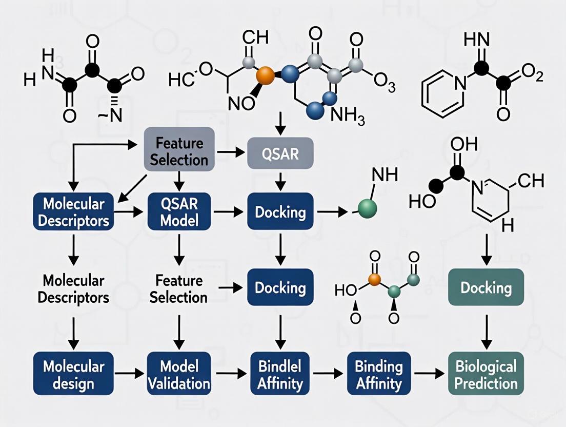
Workflow Visualization
The following diagram illustrates the integrated workflow between QSAR and molecular docking, showing how they complement each other in a drug discovery pipeline:
Integrated QSAR and Docking Workflow in Drug Discovery
Case Studies in Integrated Application
Aurora Kinase Inhibitor Development
A comprehensive study on imidazo[4,5-b]pyridine derivatives as Aurora kinase A inhibitors demonstrated the power of combining multiple QSAR techniques with docking simulations [26]. Researchers developed four different QSAR models (HQSAR, CoMFA, CoMSIA, and TopomerCoMFA) with excellent predictive statistics (cross-validation coefficients q² of 0.892-0.905), then used these models to identify key structural features influencing anticancer activity. The TopomerCoMFA model, which exhibited the highest external predictive ability (r²pred = 0.855), was particularly valuable for virtual screening of the ZINC database to identify novel R groups with potential enhanced activity [26].
Following QSAR-based design, molecular docking studies of the newly designed compounds with the Aurora A kinase structure (PDB ID: 1MQ4) helped validate binding modes and identify specific molecular interactions responsible for high affinity. This integration allowed researchers to design ten novel compounds with predicted improved activity profiles, which were further validated through molecular dynamics simulations and ADMET prediction [26].
Table 2: Key Research Reagent Solutions for Integrated QSAR-Docking Studies
| Reagent/Category | Specific Examples | Function in Research |
|---|---|---|
| Molecular Modeling Software | SYBYL2.0, Gaussian 09W, SCIGRESS, RDKit [26] [24] [29] | Compound structure building, optimization, and descriptor calculation |
| Descriptor Calculation Tools | DRAGON, PaDEL, ChemOffice [2] [24] | Computation of molecular descriptors for QSAR model development |
| Protein Structure Databases | Protein Data Bank (PDB) [26] [29] | Source of 3D protein structures for molecular docking targets |
| Chemical Databases | ZINC Database [26] | Source of commercially available compounds for virtual screening |
| Docking Platforms | AutoDock, Molecular Operating Environment (MOE) [24] [29] | Prediction of ligand-protein interactions and binding affinities |
| Dynamics Simulation Packages | GROMACS, AMBER, Desmond [26] [24] | Assessment of complex stability and interaction persistence over time |
Tubulin Inhibitors for Breast Cancer Therapy
In the development of 1,2,4-triazine-3(2H)-one derivatives as tubulin inhibitors for breast cancer treatment, researchers employed an integrated computational approach that highlighted the complementary nature of QSAR and docking [24]. The QSAR model, developed with DFT-calculated descriptors, achieved a predictive accuracy (R²) of 0.849 and identified absolute electronegativity and water solubility as key determinants of inhibitory activity. This provided quantitative guidelines for molecular design, which were then contextualized through docking studies that revealed how the most promising compound (Pred28) achieved a high binding affinity (-9.6 kcal/mol) through specific interactions with the tubulin colchicine binding site [24].
The docking results complemented the QSAR predictions by providing structural insights into why certain electronic properties enhanced activity - specifically how electronegativity features enabled optimal hydrogen bonding and hydrophobic interactions with key residues. Molecular dynamics simulations further strengthened this integration by demonstrating the stability of these interactions over time, with Pred28 showing the lowest RMSD (0.29 nm) during 100 ns simulations [24].
Coronavirus Polymerase Inhibitor Screening
A study on human coronavirus polymerase inhibitors showcased how QSAR and docking can be combined for repurposing existing nucleoside analogs [29]. Researchers calculated QSAR parameters including frontier orbital energies (HOMO-LUMO gap), electron affinity, and solvation properties for four anti-HCV drugs (Sofosbuvir, IDX-184, R7128, and MK-0608) and compared them to native nucleotides and Ribavirin. The QSAR analysis revealed that IDX-184 possessed electronic properties favorable for polymerase inhibition, which was subsequently confirmed through docking studies against 19 coronavirus polymerase models [29].
This combined approach demonstrated that IDX-184 would likely show superior binding compared to Ribavirin against MERS-CoV polymerase, while MK-0608 showed comparable performance. The synergy here allowed researchers to rapidly prioritize candidates for experimental testing without synthesizing new compounds, highlighting the efficiency gains possible through integrated computational approaches [29].
Experimental Protocols for Integrated Workflows
Protocol 1: Combined QSAR and Docking for Lead Optimization
This protocol outlines the steps for implementing an integrated QSAR-docking approach to optimize lead compounds, based on methodologies successfully applied in recent studies [26] [24] [27]:
Dataset Curation and Preparation
- Collect a structurally related compound series with measured biological activities (IC50 or Ki values)
- Convert activity values to pIC50 (-logIC50) for model development
- Divide compounds into training and test sets (typically 80:20 ratio) using rational selection methods to ensure representative chemical space coverage [24]
Molecular Descriptor Calculation and Selection
- Generate optimized 3D structures using molecular mechanics (MMFF94 or Tripos force field) followed by quantum chemical refinement (DFT with B3LYP/6-31G) [24]
- Calculate diverse molecular descriptors including:
- Apply feature selection techniques (genetic algorithm, stepwise regression) to identify most relevant descriptors [30]
QSAR Model Development and Validation
- Develop multiple QSAR models using various algorithms (MLR, PLS, RF, SVM) [2] [27]
- Validate models using both internal (cross-validation, q²) and external validation (predictions on test set, r²pred) [26]
- Apply strict validation criteria: q² > 0.5 and r²pred > 0.6 for predictive models [26]
- Interpret model coefficients to identify structural features favoring activity
Structure-Based Validation through Docking
- Prepare protein structure (from PDB or homology modeling) by adding hydrogens, assigning charges, and optimizing hydrogen bonds [26] [29]
- Define binding site based on known ligand or catalytic residues
- Dock training set compounds to verify that predicted active compounds show favorable binding interactions
- Use consensus scoring from multiple scoring functions to improve binding affinity predictions
Virtual Screening and Compound Design
- Apply validated QSAR model to screen virtual compound libraries
- Select top-ranked compounds for docking studies to verify binding mode feasibility
- Analyze docking poses to identify key protein-ligand interactions (hydrogen bonds, hydrophobic contacts, π-π stacking)
- Design new compounds by incorporating favorable structural features identified from both QSAR and docking
Experimental Validation and Iterative Refinement
- Synthesize and test top-predicted compounds
- Incorporate new experimental data to refine QSAR models
- Use iterative cycles of prediction and validation to optimize lead compounds
Protocol 2: 3D-QSAR Guided by Docking Pose Alignment
This specialized protocol is particularly useful when developing 3D-QSAR models that require spatial alignment of molecules, with docking providing the alignment rule [28]:
Binding Conformation Generation
- Dock each compound in the dataset to the target protein using flexible docking protocols
- Select the predominant binding pose for each compound based on clustering analysis and interaction consistency
- Extract the bound conformation for use in molecular alignment
Molecular Alignment for 3D-QSAR
- Align compounds using three different methods:
- Receptor-based alignment: Use docking poses directly
- Ligand-based alignment: Align to a common scaffold or pharmacophore
- Common substructure alignment: Identify maximum common substructure for alignment
- Evaluate which alignment method produces the most predictive 3D-QSAR model [28]
- Align compounds using three different methods:
3D-QSAR Model Development
- Calculate CoMFA (steric and electrostatic) and CoMSIA (additional hydrophobic, H-bond donor/acceptor) fields [26] [28]
- Use Partial Least Squares (PLS) regression to correlate field values with biological activity
- Generate 3D contour maps to visualize regions where specific molecular properties enhance or diminish activity
Model Application and Design
- Use contour maps to guide molecular modifications
- Design new compounds that incorporate favorable steric, electrostatic, and hydrophobic features indicated by the 3D-QSAR model
- Verify that designed compounds maintain complementary binding interactions identified through docking
The synergistic integration of QSAR and molecular docking represents a powerful paradigm in modern drug discovery, effectively bridging ligand-based and structure-based approaches [2] [25]. This complementary relationship enables researchers to leverage the predictive power of QSAR models with the mechanistic insights provided by docking simulations, creating a more comprehensive framework for compound optimization [26] [24]. As both methodologies continue to advance through incorporation of machine learning and improved force fields [2] [31], their integration will become increasingly seamless and impactful. The case studies and protocols presented here provide a roadmap for researchers seeking to implement this synergistic approach in their drug discovery efforts, potentially accelerating the identification and optimization of novel therapeutic agents across multiple disease areas.
Virtual screening and lead optimization represent two pivotal phases in modern computer-aided drug discovery, significantly reducing time and costs associated with bringing new therapeutics to market [32]. Virtual screening serves as a preliminary filtering technology to identify bioactive compounds from extensive chemical libraries, functioning as a complementary approach to high-throughput screening [33]. Once potential hits are identified, lead optimization focuses on improving their characteristics, including target selectivity, biological activity, potency, and toxicity profiles [34]. Within this framework, quantitative structure-activity relationship (QSAR) studies and molecular docking have emerged as indispensable computational tools that provide rational guidance for structural modification and efficacy enhancement [33] [35]. This application note details standardized protocols and practical considerations for implementing these methodologies within drug discovery pipelines.
Virtual Screening: Approaches and Applications
Virtual screening (VS) involves the in silico screening of compound libraries to identify molecules most likely to bind to a specific drug target [32]. It has become a cornerstone of modern drug discovery due to its ability to efficiently explore vast chemical spaces that would be prohibitively expensive and time-consuming to assay experimentally [36].
Key Virtual Screening Approaches
There are two primary VS approaches, which can be used independently or in combination:
Table 1: Comparison of Virtual Screening Approaches
| Approach | Description | Data Requirements | Key Advantages |
|---|---|---|---|
| Structure-Based Virtual Screening | Uses 3D structural information of the target protein to identify compounds that complement the binding site [32] | High-resolution protein structure (X-ray, NMR, or cryo-EM); homology models [32] [37] | Can identify novel scaffolds; provides structural insights for optimization |
| Ligand-Based Virtual Screening | Utilizes known active ligands to search for structurally or pharmacologically similar compounds [32] [33] | Bioactivity data of known ligands; molecular descriptors/fingerprints [38] | Effective when protein structure is unavailable; leverages existing structure-activity data |
| Pharmacophore-Based Screening | Identifies compounds containing essential steric and electronic features for optimal target interactions [32] [39] | Either protein structure or known active ligands | Abstract representation allows scaffold hopping to novel chemotypes |
Quantitative Insights and Performance Metrics
Analysis of published virtual screening results between 2007-2011 revealed that hit identification criteria vary significantly across studies [40]. Only approximately 30% of studies reported a clear, predefined hit cutoff, with no clear consensus on selection criteria. The distribution of activity cutoffs used in these studies demonstrates practical considerations for hit selection:
- 1-25 μM: 136 studies (most common range)
- 25-50 μM: 54 studies
- 50-100 μM: 51 studies
- 100-500 μM: 56 studies
- >500 μM: 25 studies (typically fragment-based screens) [40]
Modern implementations combining machine learning with traditional methods show remarkable efficiency improvements. One recent study demonstrated a 1000-fold acceleration in binding energy predictions compared to classical docking-based screening when using machine learning approaches [36].
Experimental Protocols
Protocol 1: Structure-Based Pharmacophore Modeling and Virtual Screening
This protocol generates pharmacophore models from protein-ligand structural data for virtual screening [32].
Software Requirements: Molecular Operating Environment (MOE), Discovery Studio, or similar package with pharmacophore modeling capabilities.
Procedure:
Protein Structure Preparation
- Obtain 3D structure from Protein Data Bank (PDB) or via homology modeling [32] [37]. ALPHAFOLD2 can generate reliable protein structures if experimental ones are unavailable [32].
- Add hydrogen atoms, assign protonation states, and correct any missing residues or atoms [32].
- Conduct energy minimization to relieve steric clashes.
Binding Site Characterization
- If the structure contains a bound ligand, define the binding site around this ligand.
- For apo structures, use binding site detection tools (e.g., GRID, LUDI) to identify potential binding pockets based on geometric and energetic properties [32].
Pharmacophore Feature Generation
- Analyze interactions between the protein and bound ligand (or binding site residues).
- Map key interaction features: hydrogen bond donors (HBD), hydrogen bond acceptors (HBA), hydrophobic areas (H), positively/negatively ionizable groups (PI/NI), and aromatic rings (AR) [32].
- Add exclusion volumes (XVOL) to represent the physical boundaries of the binding pocket [32].
Feature Selection and Model Validation
- Select features most critical for binding affinity, removing redundant or less important features [32].
- Validate the model using known active and inactive compounds to ensure it discriminates effectively.
Virtual Screening Implementation
- Apply the pharmacophore model as a query to screen compound databases using a search algorithm (e.g., MOE's pharmacophore search) [39].
- Generate multiple conformations for each database compound to account for flexibility.
- Retain compounds that match the pharmacophore features within defined spatial constraints.
The following workflow diagram illustrates this structure-based pharmacophore screening process:
Protocol 2: Molecular Docking for Lead Optimization
This protocol employs molecular docking to guide lead optimization through structure-activity relationship (SAR) analysis [37].
Software Requirements: Docking software (GOLD, AutoDock, Smina), molecular visualization tool (PyMOL, Chimera).
Procedure:
Structural Data Preparation and Validation
- Select high-resolution protein structure (<2.5 Å recommended) from PDB [37].
- Examine electron density maps to identify flexible or poorly resolved regions.
- Prepare protein by adding hydrogens, assigning charges, and removing water molecules (unless functionally important).
Ligand Preparation
- Generate 3D structures of lead compounds and analogs.
- Assign proper protonation states at physiological pH.
- Perform energy minimization using appropriate force fields.
Docking Workflow Establishment
- Define binding site coordinates based on known ligand position or active site residues.
- Select docking algorithm (genetic algorithm, Monte Carlo) and scoring function appropriate for your target [37].
- Validate docking protocol by re-docking known ligands and reproducing experimental binding poses (RMSD < 2.0 Å).
SAR Analysis and Compound Prioritization
- Dock series of analog structures to explore structure-activity relationships.
- Analyze binding modes to identify key interactions contributing to affinity.
- Correlate docking scores with experimental activities to validate predictive capability.
Interaction Mapping for Design
- Identify suboptimal interactions in current leads that could be improved.
- Propose structural modifications to enhance complementary interactions.
- Design new analogs with improved potency or selectivity.
The lead optimization process informed by docking and SAR analysis follows an iterative cycle:
Protocol 3: Machine Learning-QSAR Model Development
This protocol develops robust 2D QSAR models using machine learning to predict compound activity [38] [35].
Software Requirements: Python with scikit-learn, PaDEL descriptor software, KNIME, or other cheminformatics platforms.
Procedure:
Dataset Curation
Molecular Descriptor Calculation and Feature Selection
Model Training and Validation
- Split data into training (80%) and test (20%) sets, ensuring representative chemical space coverage [38].
- Train multiple ML algorithms: Support Vector Machine (SVM), Artificial Neural Network (ANN), and Random Forest (RF) [38].
- Optimize hyperparameters for each algorithm using grid search and cross-validation.
Model Evaluation and Selection
Model Application for Prediction
- Use the validated model to predict activities of virtual compound libraries.
- Apply ADMET filters to prioritize compounds with favorable drug-like properties [38].
- Select top-ranked compounds for further experimental validation.
The Scientist's Toolkit: Essential Research Reagent Solutions
Table 2: Key Research Reagents and Computational Tools for Virtual Screening and Lead Optimization
| Category | Specific Tools/Resources | Function and Application |
|---|---|---|
| Structural Databases | Protein Data Bank (PDB) [37] | Repository of 3D protein structures for structure-based design |
| Compound Libraries | ZINC Database [36] | Commercially available compounds for virtual screening |
| Bioactivity Data | ChEMBL Database [36] [38] | Curated bioactivity data for ligand-based design and QSAR modeling |
| Docking Software | GOLD, AutoDock, Smina [37] [36] | Predict binding poses and scores for protein-ligand complexes |
| Pharmacophore Modeling | MOE, Discovery Studio [39] | Create and screen pharmacophore models for virtual screening |
| Descriptor Calculation | PaDEL [38] | Compute molecular descriptors and fingerprints for QSAR |
| Machine Learning Libraries | scikit-learn [38] | Implement ML algorithms for QSAR and activity prediction |
Virtual screening and lead optimization represent interconnected pillars of modern computational drug discovery. Structure-based approaches leveraging pharmacophore modeling and molecular docking provide mechanistic insights for compound design [32] [37], while ligand-based QSAR strategies efficiently leverage existing structure-activity data to guide optimization [38] [35]. The integration of machine learning methodologies across these domains offers unprecedented acceleration, enabling more effective navigation of chemical space and enhanced prediction of compound properties [41] [36]. By implementing the standardized protocols outlined in this application note, researchers can establish robust computational workflows that significantly enhance efficiency in identifying and optimizing novel therapeutic candidates.
From Theory to Practice: Implementing QSAR and Docking Methodologies
Molecular descriptors are mathematical representations of a molecule's structural, physicochemical, and electronic properties that form the foundational variables in Quantitative Structure-Activity Relationship (QSAR) modeling [42] [43]. The selection of appropriate descriptors is a critical step in building robust QSAR models, as they quantitatively encode chemical information that can be correlated with biological activity [10]. Descriptors are typically classified by dimensionality—1D, 2D, 3D, and 4D—based on the level of structural information they encode, with each category offering distinct advantages for specific applications in drug discovery [2] [43]. The evolution of QSAR from classical linear models to sophisticated machine learning and deep learning frameworks has further emphasized the importance of strategic descriptor selection to capture complex, nonlinear patterns across large chemical spaces [2] [10]. This protocol provides a comprehensive guide to the classification, calculation, and application of molecular descriptors within modern QSAR workflows, with particular emphasis on integration with molecular docking studies.
Molecular Descriptor Classification and Characteristics
Molecular descriptors can be broadly categorized by dimensionality, with each level incorporating increasingly complex structural information. The table below summarizes the key descriptor types, their characteristics, and primary applications in drug discovery research.
Table 1: Classification of Molecular Descriptors by Dimensionality
| Descriptor Type | Structural Information Encoded | Example Descriptors | Computational Cost | Primary Applications |
|---|---|---|---|---|
| 1D Descriptors | Bulk properties & whole-molecule characteristics | Molecular weight, log P, atom counts, polar surface area [43] [44] | Low | Preliminary screening, ADMET prediction [44] |
| 2D Descriptors | Structural fragments & molecular connectivity | Topological indices, connectivity fingerprints, graph-based descriptors [2] [43] | Low to Moderate | High-throughput virtual screening, similarity searching [45] [43] |
| 3D Descriptors | Molecular shape, surface, & volume properties | Molecular surface area, volume, 3D-MoRSE descriptors, WHIM descriptors [2] [45] | Moderate to High | Ligand-protein docking, binding affinity prediction [45] [46] |
| 4D Descriptors | Conformational flexibility & ensemble properties | Ensemble-averaged spatial features, grid-based occupancy [2] | High | Incorporating flexibility in binding site interactions [2] |
| Quantum Chemical Descriptors | Electronic structure & reactivity properties | HOMO-LUMO energies, dipole moment, electrostatic potential surfaces [2] | Very High | Modeling reaction pathways & electronic interactions [2] |
Experimental Protocols for Descriptor Calculation and Application
Protocol 1: Comprehensive Descriptor Generation Workflow
Objective: To generate a multi-dimensional descriptor set for QSAR model development.
Materials and Software:
- Chemical Structures: Standardized molecular structures in SDF, MOL2, or SMILES format [42]
- Descriptor Calculation Software: RDKit, PaDEL-Descriptor, Dragon, Mordred, or Schrödinger's DeepAutoQSAR [2] [42] [47]
- Computational Environment: Workstation with multi-core processor (≥16 GB RAM recommended for 3D/4D descriptors)
Procedure:
- Data Preprocessing:
Descriptor Calculation:
- 1D/2D Descriptors: Process structures through RDKit or PaDEL-Descriptor to calculate constitutional, topological, and electronic descriptors [42] [44].
- 3D Descriptors: Use Dragon or Schrödinger Maestro to compute steric, surface, and shape descriptors from energy-minimized 3D structures [2] [45].
- Quantum Chemical Descriptors: Perform geometry optimization and orbital calculation using Gaussian, GAMESS, or Schrödinger Jaguar at appropriate theory levels (e.g., B3LYP/6-31G*) [2].
- 4D Descriptors: Generate conformational ensembles using molecular dynamics simulations (e.g., 1-10ns in explicit solvent) and calculate ensemble-averaged spatial descriptors [2].
Descriptor Preprocessing:
- Remove constant and near-constant descriptors (variance threshold <0.01).
- Eliminate highly correlated descriptors (pairwise correlation >0.95).
- Apply standardization (z-score normalization) to scale descriptors for machine learning [42].
Figure 1: Comprehensive Workflow for Molecular Descriptor Generation and Preprocessing
Protocol 2: Comparative Evaluation of Descriptor Sets for ADME-Tox Prediction
Objective: To systematically compare the performance of different descriptor types in predicting ADME-Tox endpoints.
Experimental Design:
- Datasets: Curated ADME-Tox datasets (≥1,000 compounds) for endpoints like Ames mutagenicity, hERG inhibition, BBB permeability [44]
- Descriptor Sets: 1D, 2D, 3D descriptors; Morgan, MACCS, Atompairs fingerprints [44]
- Machine Learning Algorithms: XGBoost and RPropMLP neural networks [44]
- Validation: 5-fold cross-validation with external test set (80/20 split) [42]
Procedure:
- Dataset Curation:
Model Building and Evaluation:
Statistical Analysis:
- Compare performance across descriptor types using ANOVA with post-hoc tests.
- Identify optimal descriptor combinations for each ADME-Tox endpoint.
Table 2: Performance Comparison of Descriptor Types in ADME-Tox Prediction (Based on [44])
| ADME-Tox Endpoint | Best Performing Descriptor Type | Alternative Performers | Key Findings |
|---|---|---|---|
| Ames Mutagenicity | 2D Descriptors | 1D Descriptors, Combined Sets | 2D descriptors outperformed fingerprints in prediction accuracy [44] |
| hERG Inhibition | 2D Descriptors | 3D Descriptors, Morgan Fingerprints | Traditional 2D descriptors showed superior performance with XGBoost [44] |
| BBB Permeability | 2D Descriptors | 3D Descriptors, MACCS | 2D descriptors produced better models than combined descriptor sets [44] |
| P-glycoprotein Inhibition | 3D Descriptors | 2D Descriptors, Atompairs | Shape and volume descriptors contributed significantly to inhibition prediction |
| Hepatotoxicity | Combined 2D+3D Descriptors | 2D Descriptors Alone | Complementary information from 2D and 3D descriptors enhanced prediction [45] |
| CYP 2C9 Inhibition | 2D Descriptors | Morgan Fingerprints | Electronic and topological descriptors captured essential inhibition mechanisms |
Integration of Molecular Descriptors with Molecular Docking
Protocol 3: Hybrid QSAR-Docking Approach for Virtual Screening
Objective: To combine molecular descriptor-based QSAR with molecular docking for enhanced virtual screening.
Materials and Software:
- Protein Preparation: Protein Data Bank structures, prepared using Schrödinger's Protein Preparation Wizard or similar [46]
- Docking Software: Glide, AutoDock Vina, GOLD, or FlexX [46] [16]
- QSAR Software: Scikit-learn, DeepAutoQSAR, or custom machine learning pipelines [2] [47]
Procedure:
- Initial Screening with QSAR Models:
- Develop validated QSAR models using optimal descriptor combinations from Protocol 2.
- Screen large compound libraries (1M+ compounds) using the QSAR model to identify top candidates (0.1-1% of library).
Molecular Docking of QSAR-Prioritized Compounds:
- Prepare protein target: remove water molecules, add hydrogens, optimize hydrogen bonding networks [46].
- Define binding site using co-crystallized ligand or known active site residues.
- Dock QSAR-prioritized compounds using multiple docking programs (Glide, AutoDock Vina) for consensus [46] [16].
- Validate docking protocol by re-docking native ligand (target RMSD <2.0 Å) [46].
Binding Affinity Refinement with Quantum Chemical Descriptors:
- For top-ranked docked poses (50-100 compounds), calculate quantum chemical descriptors (HOMO-LUMO gap, molecular orbital energies, electrostatic potentials) [2].
- Correlate quantum descriptors with binding scores to identify electronic features enhancing binding.
Consensus Scoring and Prioritization:
- Develop consensus scoring combining docking scores, QSAR predictions, and quantum chemical properties.
- Select final compounds (20-50) for experimental validation based on multi-parameter optimization.
Figure 2: Integrated QSAR-Docking Workflow for Virtual Screening
Research Reagent Solutions: Essential Tools for Descriptor Calculation
Table 3: Essential Software and Tools for Molecular Descriptor Calculation
| Tool Name | Descriptor Types Supported | Key Features | Application Context |
|---|---|---|---|
| RDKit | 1D, 2D, Fingerprints | Open-source, Python integration, extensive cheminformatics toolkit [42] [43] | Academic research, prototype QSAR model development |
| PaDEL-Descriptor | 1D, 2D, Fingerprints | 1D/2D descriptors and fingerprints, user-friendly interface [2] [42] | High-throughput descriptor calculation for large datasets |
| Dragon | 1D, 2D, 3D, 4D | Comprehensive descriptor coverage (5,000+ descriptors), well-validated [2] | Professional QSAR modeling requiring diverse descriptor types |
| Schrödinger DeepAutoQSAR | 1D, 2D, 3D, ML descriptors | Automated machine learning, uncertainty estimation, graph neural networks [47] | Industrial drug discovery with large-scale QSAR modeling |
| AutoDock Vina | Docking-specific descriptors | Fast docking, good performance in binding pose prediction [46] [16] | Structure-based virtual screening and binding pose prediction |
| Gaussian | Quantum Chemical Descriptors | Ab initio calculations, DFT methods, orbital energy calculations [2] | High-accuracy electronic property calculation for lead optimization |
Strategic selection of molecular descriptors is paramount for developing predictive QSAR models in drug discovery. The experimental protocols outlined demonstrate that 2D descriptors frequently provide optimal performance for ADME-Tox prediction, while 3D and quantum chemical descriptors add value for specific binding interactions [45] [44]. The integration of descriptor-based QSAR with molecular docking creates a powerful hybrid approach that leverages the strengths of both ligand-based and structure-based methods [2] [46]. As QSAR evolves with advances in artificial intelligence, modern deep learning approaches are increasingly utilizing learned molecular representations that automatically extract relevant features from molecular structures [2] [48]. However, understanding the fundamental principles of molecular descriptor selection remains essential for constructing validated, interpretable QSAR models that effectively guide drug discovery optimization.
In modern drug discovery, Quantitative Structure-Activity Relationship (QSAR) modeling serves as a cornerstone for predicting compound activity and optimizing lead molecules. The evolution from classical statistical methods to modern machine learning (ML) and deep learning (DL) frameworks has transformed computational pipelines, enabling faster and more accurate prediction of compound properties [2]. This paradigm shift is critical within the broader context of integrated computational approaches, where QSAR synergizes with molecular docking and molecular dynamics (MD) simulations to provide comprehensive insights into ligand-target interactions and accelerate the identification of viable drug candidates [49] [2]. Understanding the strengths, limitations, and appropriate application domains of classical versus machine learning approaches is therefore essential for researchers, scientists, and drug development professionals aiming to build robust predictive models.
Theoretical Foundations and Evolution of QSAR Modeling
The fundamental principle of QSAR modeling is to establish a mathematical relationship between the chemical structure of compounds and their biological activity or physicochemical properties. This is achieved through the use of molecular descriptors—numerical representations that encode various aspects of molecular structure and properties [2]. Descriptors are broadly categorized by dimensions:
- 1D descriptors include global molecular properties such as molecular weight and atom count.
- 2D descriptors (topological descriptors) capture structural patterns and connectivity, such as topological indices.
- 3D descriptors convey information about molecular shape, surface, and electrostatic potential maps.
- 4D descriptors account for conformational flexibility by considering ensembles of molecular structures.
- Quantum chemical descriptors, such as HOMO-LUMO energy gaps and dipole moments, describe electronic properties crucial for interactions with biological targets [2].
The evolution of QSAR modeling reflects a journey from interpretable linear models to complex nonlinear algorithms capable of handling high-dimensional chemical spaces. Classical QSAR methods emerged from foundational work by Hansch and Fujita, utilizing linear regression techniques to relate descriptors to activity [50]. The machine learning era introduced algorithms capable of capturing intricate, nonlinear patterns in large, diverse datasets, with recent advances incorporating deep learning and graph neural networks (GNNs) that learn molecular representations directly from structure data without manual feature engineering [2]. This progression has significantly expanded the scope and predictive power of QSAR modeling in contemporary drug discovery pipelines.
Classical Statistical Methods in QSAR
Core Principles and Techniques
Classical QSAR modeling relies on statistical regression techniques to correlate a set of molecular descriptors with a biological endpoint. These methods are grounded in linear algebra and assume a linear or linearizable relationship between the independent variables (descriptors) and the dependent variable (biological activity). The most prominent techniques include:
- Multiple Linear Regression (MLR): Establishes a linear relationship between multiple independent variables and the response variable. It is valued for its simplicity and high interpretability, as coefficients directly indicate the contribution of each descriptor.
- Partial Least Squares (PLS): Particularly effective when descriptors are numerous and highly collinear (correlated). PLS projects both descriptors and response variables into a new, lower-dimensional space of latent variables that maximize the covariance between them.
- Principal Component Regression (PCR): Similar to PLS, PCR uses principal component analysis (PCA) to transform the original descriptors into a set of uncorrelated principal components, which are then used as predictors in a regression model.
These methods are often complemented by rigorous feature selection techniques to identify the most relevant descriptors and reduce the risk of overfitting. Common approaches include stepwise regression, genetic algorithms, and filter methods based on correlation coefficients [50].
Experimental Protocol for Classical QSAR Modeling
Objective: To construct a predictive classical QSAR model using Multiple Linear Regression (MLR) and Partial Least Squares (PLS) regression.
Materials and Data Requirements:
- A curated set of compounds with experimentally measured biological activity (e.g., IC₅₀, Ki).
- Calculated molecular descriptors (e.g., using DRAGON, PaDEL, or RDKit).
- Statistical software (e.g., QSARINS, Build QSAR, or R/Python with relevant libraries).
Procedure:
Data Curation and Preparation
- Compound structures should be standardized (e.g., neutralize charges, remove duplicates).
- Biological activity values (e.g., IC₅₀) are converted to a molar scale and transformed into pIC₅₀ (-log₁₀IC₅₀) to ensure a linear relationship with free energy changes.
- Calculate a comprehensive set of molecular descriptors for all compounds.
Descriptor Pre-screening and Data Set Preparation
- Remove descriptors with zero or near-zero variance.
- Use pairwise correlation analysis (e.g., calculating the coefficient of determination, CoD, between descriptors) to eliminate highly correlated redundant descriptors. A common threshold is a CoD > 0.95 [50].
- Split the data into a training set (~70-80%) for model building and a test set (~20-30%) for external validation.
Model Development and Training
- For MLR: Use feature selection methods (e.g., stepwise selection, Genetic Function Algorithm (GFA)) on the training set to identify a subset of descriptors that yield a statistically significant model.
- For PLS: The optimal number of latent components is determined via cross-validation on the training set to avoid overfitting.
Model Validation
- Internal Validation: Assess model robustness using techniques like Leave-One-Out (LOO) or Leave-Group-Out (LGO) cross-validation. Report the cross-validated R² (Q²) and Root Mean Square Error (RMSE).
- External Validation: Predict the activity of the test set compounds. Calculate the coefficient of determination for the external test set (R²ext) and its RMSE.
- Y-Randomization: Perform multiple random shuffles of the response variable to ensure the model is not based on chance correlation.
Model Interpretation and Applicability Domain
- Analyze the magnitude and sign of coefficients in MLR to interpret the physicochemical influence of each descriptor on the activity.
- Define the model's Applicability Domain (AD) using approaches like the William's plot (leverage vs. standardized residuals) to identify compounds for which predictions are reliable.
Applications and Case Studies
Classical QSAR remains highly relevant in specific contexts. For instance, Olenginski et al. applied QSAR to understand the structural determinants of RNA-binding small molecules [2]. In another study, researchers utilized 2D-QSAR, molecular docking, and ADMET profiling to design blood-brain barrier permeable BACE-1 inhibitors for Alzheimer's disease, demonstrating the integration of classical QSAR within a broader drug discovery pipeline [2]. Its strengths lie in preliminary screening, lead optimization, and scenarios where model interpretability is paramount, such as in regulatory toxicology for REACH compliance [2].
Machine Learning Approaches in QSAR
Core Algorithms and Workflow
Machine learning has markedly expanded the capabilities of QSAR by enabling the modeling of complex, non-linear relationships in high-dimensional data. Key algorithms include:
- Random Forests (RF): An ensemble method that constructs multiple decision trees and aggregates their results. It is robust to noisy data and inherently performs feature selection, making it a popular choice for cheminformatics [2].
- Support Vector Machines (SVM): Effective in high-dimensional spaces, SVMs find a hyperplane that best separates active from inactive compounds. They are particularly useful when the number of descriptors exceeds the number of samples.
- k-Nearest Neighbors (kNN): A simple, instance-based algorithm that predicts activity based on the activities of the most similar compounds in the descriptor space.
- Advanced Deep Learning (DL): This includes Graph Neural Networks (GNNs), which operate directly on molecular graph structures, and models that process SMILES strings, such as transformers. These methods automate feature representation learning, capturing hierarchical chemical features without manual descriptor engineering [2].
The ML-QSAR workflow emphasizes robust validation and interpretability. Techniques like SHAP (SHapley Additive exPlanations) and LIME (Local Interpretable Model-agnostic Explanations) are increasingly used to interpret "black-box" models by quantifying the contribution of individual descriptors to predictions [2].
Experimental Protocol for Machine Learning QSAR Modeling
Objective: To develop a predictive QSAR model using a machine learning algorithm (e.g., Random Forest) and validate its performance and applicability.
Materials and Data Requirements:
- A curated data set of compounds and their biological activities.
- Calculated molecular descriptors or learned molecular representations (e.g., from GNNs).
- Programming environment with ML libraries (e.g., scikit-learn, KNIME, AutoQSAR in Python/R).
Procedure:
Data Curation and Preparation
- Follow the same data standardization and pIC₅₀/pKᵢ transformation steps as in the classical protocol.
- Calculate traditional molecular descriptors or generate latent representations using a deep learning model.
Data Set Splitting and Feature Pre-processing
- Partition data into training, validation (optional), and test sets. Stratified splitting is recommended for classification tasks to maintain class distribution.
- Scale descriptors (e.g., standardization or normalization) to ensure algorithms that rely on distance metrics are not biased.
Model Training and Hyperparameter Optimization
- Train the selected ML algorithm (e.g., Random Forest) on the training set.
- Use techniques like grid search or Bayesian optimization with cross-validation on the training set to tune hyperparameters (e.g., number of trees in RF, kernel type in SVM).
Model Validation
- Internal Validation: Use k-fold cross-validation (e.g., 5-fold) on the training set to estimate model performance and stability. Report Q² and RMSE.
- External Validation: The final model, trained on the entire training set with optimized hyperparameters, is used to predict the held-out test set. Report R²ext, RMSE, and for classification, metrics like balanced accuracy, sensitivity, and specificity [51].
- For classification models, a threshold (e.g., 1 μM) is used to bin compounds into active/inactive categories [51].
Model Interpretation and Deployment
- Use interpretability tools like SHAP to identify the most important molecular features driving the predictions.
- Define the applicability domain of the model using approaches such as leverage or distance-based methods in the descriptor space.
- Deploy the validated model for virtual screening of large chemical libraries.
Applications and Performance Benchmarks
Machine learning excels in virtual screening and managing large, complex datasets. A notable benchmark from the 2025 ASAP-Polaris-OpenADMET Antiviral Challenge revealed that while classical methods remain competitive for predicting compound potency, modern deep learning algorithms significantly outperformed traditional machine learning in ADME (Absorption, Distribution, Metabolism, and Excretion) prediction [52]. Furthermore, a comparative study on predicting interactions with anti-targets found that qualitative SAR models showed higher balanced accuracy (0.80-0.81) than quantitative QSAR models (0.73-0.76), though QSAR models exhibited higher specificity [51].
Comparative Analysis: Classical vs. Machine Learning QSAR
The choice between classical and machine learning approaches for QSAR modeling depends on the specific problem, data characteristics, and project goals. The table below summarizes the key differences.
Table 1: Comparative analysis of classical statistical methods and machine learning approaches in QSAR modeling.
| Aspect | Classical Statistical Methods | Machine Learning Approaches |
|---|---|---|
| Core Algorithms | Multiple Linear Regression (MLR), Partial Least Squares (PLS), Principal Component Regression (PCR) [2] | Random Forest (RF), Support Vector Machines (SVM), k-Nearest Neighbors (kNN), Graph Neural Networks (GNNs) [2] |
| Model Interpretability | High; descriptor coefficients provide direct physicochemical insight [2] | Lower (often "black-box"); requires post-hoc tools (SHAP, LIME) for interpretation [2] |
| Handling of Non-linearity | Poor; assumes linear relationships | Excellent; capable of modeling complex, non-linear patterns [2] |
| Data Efficiency | Effective with smaller datasets (tens to hundreds of compounds) | Requires larger datasets (hundreds to thousands of compounds) for robust performance |
| Feature Selection | Often requires explicit pre-screening (e.g., correlation analysis [50]) | Many algorithms (e.g., RF) have built-in feature importance assessment [2] |
| Typical Performance | Competitive for potency prediction with well-behaved data [52] | Superior for complex endpoint prediction (e.g., ADME) [52] |
| Primary Application Context | Preliminary screening, mechanistic interpretation, regulatory toxicology (REACH) [2] | Virtual screening of large libraries, complex ADMET endpoint prediction, de novo drug design [2] |
Integrated Workflow in Drug Discovery
QSAR models are rarely used in isolation. They are most powerful when integrated into a cohesive drug discovery workflow that includes structure-based modeling techniques. The following diagram illustrates a modern, integrated computational pipeline that leverages both ligand-based (QSAR) and structure-based methods for comprehensive candidate evaluation.
Integrated QSAR and Molecular Modeling Workflow
This workflow begins with parallel ligand-based (QSAR) and structure-based (Docking) virtual screening of compound libraries. Top-ranked compounds from both approaches advance to molecular dynamics (MD) simulations to assess binding stability and interaction dynamics under physiological conditions—a step highlighted in the design of HCV NS5B polymerase inhibitors, where MD simulations confirmed stable binding of designed compounds [49]. Finally, promising candidates undergo predictive ADMET profiling to filter out compounds with poor pharmacokinetics or potential toxicity early in the discovery process [2].
The Scientist's Toolkit: Essential Research Reagents and Computational Tools
Successful QSAR modeling relies on a suite of software tools, databases, and computational resources. The following table details key components of the modern QSAR researcher's toolkit.
Table 2: Essential research reagents, software, and databases for QSAR modeling and related computational analyses.
| Tool/Resource Name | Type/Category | Primary Function in Research |
|---|---|---|
| DRAGON, PaDEL, RDKit [2] | Molecular Descriptor Calculator | Generates a wide array of 1D, 2D, and 3D molecular descriptors from compound structures. |
| QSARINS, Build QSAR [2] | Classical QSAR Software | Provides specialized environments for developing and rigorously validating classical statistical QSAR models. |
| scikit-learn, KNIME [2] | Machine Learning Platform | Offers comprehensive libraries and graphical interfaces for building, testing, and deploying ML-based QSAR models. |
| ChEMBL, PubChem [51] | Public Chemical Database | Sources of curated chemical structures and associated bioactivity data for model training and validation. |
| GUSAR [51] | (Q)SAR Modeling Software | A specialized software for creating both quantitative (QSAR) and qualitative (SAR) models using MNA and QNA descriptors. |
| AutoDock, GOLD | Molecular Docking Software | Predicts the binding orientation and affinity of a small molecule within a protein's active site. |
| Desmond, GROMACS [49] | Molecular Dynamics (MD) Software | Simulates the time-dependent dynamic behavior of protein-ligand complexes to assess binding stability. |
| SHAP, LIME [2] | Model Interpretability Tool | Provides post-hoc interpretation of complex machine learning models to identify influential molecular features. |
Molecular docking is a pivotal component of computer-aided drug design (CADD), consistently contributing to advancements in pharmaceutical research [53]. In essence, it employs computational algorithms to identify the optimal binding mode between two molecules, such as a protein receptor and a small molecule ligand, predicting the three-dimensional structure of the resulting complex [53]. This process is of particular significance for understanding the mechanistic intricacies of physicochemical interactions at the atomic scale and has wide-ranging implications for structure-based drug design [53]. The accuracy of docking predictions is fundamentally constrained by the quality of protein preparation, the precise definition of binding sites, and the sampling/scoring algorithms used for pose prediction [54] [55]. These protocols do not exist in isolation but are intrinsically linked to Quantitative Structure-Activity Relationship (QSAR) modeling, as the structural insights derived from docking complexes directly inform the molecular descriptors and mechanistic hypotheses that underpin robust QSAR models [2]. This application note details standardized protocols for these critical steps, framing them within the integrated context of modern drug discovery pipelines that leverage both structure-based and ligand-based approaches.
Protein Preparation Protocols
The preparation of the protein structure is a critical first step that significantly influences the outcome of molecular docking studies. A properly prepared model ensures computational accuracy and biological relevance.
Input Structure Acquisition and Assessment
The initial stage involves acquiring a high-quality three-dimensional structure of the target protein.
- Experimental Structures: Structures determined by X-ray crystallography, cryo-electron microscopy (cryo-EM), or NMR spectroscopy are preferred sources. The Protein Data Bank (PDB) is the primary repository for such structures [53] [56]. When evaluating a PDB entry, key parameters to consider are the resolution (with values below 2.5 Å generally desirable for X-ray structures), the completeness of the protein chain in regions of interest, and the absence of significant steric clashes [56].
- Computational Models: For targets with no experimental structure, homology models can be used. Good models can be generated with sequence identities >40% to a known template structure using programs like MODELLER, and they can be sourced from public databases such as ModBase or the Protein Model Portal [56]. The sensitivity of docking protocols to structural deviations makes the quality of the input model paramount [56]. More recently, AlphaFold-predicted structures and other deep learning-based models have shown considerable utility, though their performance may vary for specific targets like antibody-antigen complexes [57].
Standardized Preparation Workflow
A systematic protocol must be applied to the raw input structure to generate a docking-ready model. The following steps are essential, often implemented using tools within software suites like OESpruce [58]:
- Hydrogen Addition and Protonation States: Add all missing hydrogen atoms. Determine the protonation states of ionizable residues (e.g., Asp, Glu, His, Lys) at the intended physiological pH (typically 7.4). This is crucial for modeling correct hydrogen bonding and ionic interactions [53].
- Loop Modeling and Missing Side Chains: Use dedicated algorithms to model missing loops or side chains, ensuring the protein structure is complete.
- Removal of Artifacts and Water Molecules: Delete non-structural ions, solvent molecules, and co-crystallized ligands. However, structurally conserved water molecules that mediate key interactions may be retained.
- Energy Minimization: Perform a limited energy minimization to relieve steric clashes and correct distorted geometries introduced during the modeling process. This step ensures the final protein structure is energetically favorable.
The diagram below illustrates the logical workflow for the protein preparation protocol.
Key Research Reagent Solutions for Protein Preparation
Table 1: Essential software and databases for protein structure preparation.
| Research Reagent | Type | Primary Function in Preparation |
|---|---|---|
| Protein Data Bank (PDB) | Database | Repository for experimentally determined 3D structures of proteins and nucleic acids [53]. |
| MODELLER | Software | Generates homology models of protein structures based on alignment to known template structures [56]. |
| AlphaFold | Software | Predicts protein 3D structures from amino acid sequences with high accuracy, useful when experimental structures are unavailable [57]. |
| OESpruce | Software | A specialized tool for preparing protein structures from the PDB for molecular docking and virtual screening, including bond order assignment and protonation [58]. |
| pdb2pqr | Software | Prepares structures for electrostatic calculations by adding hydrogens, assigning charge states, and generating PQR files [56]. |
Binding Site Analysis and Prediction
Identifying and characterizing the binding site is a prerequisite for successful focused docking. Binding sites can be known from experimental data or predicted computationally.
Ligand-Aware Binding Site Prediction with LABind
Traditional methods often treat binding site identification as a property of the protein alone. The LABind method represents a significant advancement by explicitly incorporating ligand information in a structure-based approach to predict binding sites for small molecules and ions [55]. Its protocol can be summarized as follows:
Input Representation:
- Protein: The protein's sequence and 3D structure are input. Sequence embeddings are generated using the Ankh protein language model, while structural features (angles, distances, directions) are extracted from atomic coordinates and encoded as a graph. Secondary structure features are obtained from DSSP [55].
- Ligand: The ligand's Simplified Molecular Input Line Entry System (SMILES) string is input into the MolFormer molecular language model to obtain a numerical representation of its properties [55].
Graph-Based Feature Integration: The protein is represented as a graph where nodes are residues. A graph transformer captures potential binding patterns from the local spatial context of the protein [55].
Cross-Attention Mechanism: A core component of LABind, this mechanism learns the distinct binding characteristics between the specific protein and ligand by processing their respective representations. This allows the model to predict binding sites in a ligand-aware manner, even for ligands not seen during training [55].
Binding Residue Classification: The final output is a per-residue prediction, classifying each residue as part of a binding site or not, achieved through a multi-layer perceptron (MLP) classifier [55].
LABind has demonstrated superior performance on multiple benchmark datasets (DS1, DS2, DS3) in terms of AUC, AUPR, and MCC, and has proven effective in predicting binding site centers and distinguishing between sites for different ligands [55].
Performance Evaluation of Binding Site Prediction Methods
Table 2: Quantitative performance of LABind compared to other methods on benchmark datasets. Adapted from LABind experimental results [55].
| Method | Type | AUC (DS1) | AUPR (DS1) | AUC (DS2) | AUPR (DS2) | Key Advantage |
|---|---|---|---|---|---|---|
| LABind | Ligand-Aware | 0.94 | 0.72 | 0.92 | 0.67 | Predicts sites for unseen ligands |
| GraphBind | Single-Ligand-Oriented | 0.89 | 0.61 | 0.87 | 0.58 | Specialized for specific ligands |
| P2Rank | Multi-Ligand-Oriented | 0.87 | 0.55 | 0.85 | 0.53 | Protein-structure only |
| DeepPocket | Multi-Ligand-Oriented | 0.86 | 0.54 | 0.84 | 0.52 | Protein-structure only |
Pose Prediction and Sampling Strategies
Pose prediction involves computationally identifying the optimal binding geometry (pose) of the ligand within the protein's binding site. This process must account for both the flexibility of the ligand and, often, the protein.
Physical Basis and Sampling Algorithms
The goal of docking is to find the ligand pose that minimizes the Gibbs free energy of binding (ΔGbind) [53]. The binding free energy is governed by the enthalpic (ΔH) and entropic (TΔS) contributions of various non-covalent interactions, including hydrogen bonds, ionic interactions, Van der Waals forces, and hydrophobic effects [53]. Docking algorithms employ different sampling strategies to explore the conformational space:
- Systematic Search: Explores rotatable bonds in the ligand.
- Stochastic Search: Uses random changes to generate new poses (e.g., Monte Carlo methods, evolutionary algorithms).
- Distance-Based Constraints: Can incorporate experimental data to restrict the search space to regions known to be important for binding [56].
The pepATTRACT protocol, for instance, is designed for fully blind, flexible peptide-protein docking. It handles peptide flexibility explicitly and allows users to specify "active residues" on the protein to guide the docking search, significantly improving efficiency and accuracy [56].
Integrating Deep Learning and Physics-Based Sampling
A major challenge in pose prediction is conformational flexibility. While traditional tools like ReplicaDock 2.0 use physics-based replica exchange Monte Carlo to sample flexibility, they can be computationally intensive [57]. The AlphaRED pipeline addresses this by intelligently combining deep learning with physics-based methods:
- Initial Prediction with AlphaFold-Multimer (AFm): AFm is first used to generate structural templates of the protein complex [57].
- Confidence Evaluation: The predicted Local Distance Difference Test (pLDDT) score from AFm, especially at the putative interface, is used to assess the model's confidence [57].
- Conditional Refinement:
- Low-Confidence Prediction: If the interface pLDDT is low, indicating high flexibility or poor prediction, AlphaRED triggers global docking simulations using ReplicaDock 2.0 to extensively explore conformational space [57].
- High-Confidence Prediction: For high-confidence models, AlphaRED performs localized refinement, focusing on flexible backbone regions identified by low per-residue pLDDT scores [57].
This hybrid approach has demonstrated remarkable success, doubling the performance of AFm alone on challenging antibody-antigen targets (43% success rate vs. AFm's ~21%) and generating acceptable-quality models for 63% of benchmark targets [57].
The following diagram outlines this integrated pose prediction workflow.
Integration with QSAR in Drug Discovery
The synergy between molecular docking and QSAR modeling is a cornerstone of modern computational drug discovery. Docking provides a structural and mechanistic context for QSAR models [2]. The binding poses generated by docking can be used to calculate 3D molecular descriptors that encode information about the specific interactions at the binding site (e.g., hydrogen bond distances, hydrophobic contact surfaces) [2]. These structure-informed descriptors often lead to more robust and interpretable QSAR models than those derived from ligand-based 2D descriptors alone.
Conversely, machine learning and AI are now deeply integrated into both fields. AI-augmented QSAR methodologies use advanced algorithms like graph neural networks to capture complex, non-linear patterns in chemical data [2] [25]. Furthermore, multitask learning frameworks like DeepDTAGen exemplify the next level of integration, simultaneously predicting drug-target binding affinity (DTA) and generating novel, target-aware drug molecules using a shared feature space [59]. This unified approach directly leverages the knowledge of ligand-receptor interactions for both predictive and generative tasks, greatly accelerating the drug discovery process [59] [25].
In modern drug discovery, the integration of computational methodologies has transformed the lead identification and optimization process. Combining Quantitative Structure-Activity Relationship (QSAR) modeling, molecular docking, and ADMET (Absorption, Distribution, Metabolism, Excretion, and Toxicity) prediction creates a powerful synergistic workflow that significantly accelerates candidate screening while reducing reliance on costly experimental approaches [60] [61]. These integrated pipelines enable researchers to rapidly identify promising therapeutic candidates with desirable biological activity and favorable pharmacokinetic profiles early in the discovery process [62] [63]. The evolution of these approaches from basic linear models to advanced machine learning (ML) and deep learning (DL) frameworks has further enhanced their predictive accuracy and applicability across diverse chemical spaces [61] [5] [63]. This application note details established protocols and best practices for implementing these integrated computational workflows, providing researchers with practical frameworks for efficient drug discovery campaigns.
The synergistic combination of QSAR, docking, and ADMET prediction creates a comprehensive computational pipeline that systematically progresses from initial compound screening to detailed binding interaction analysis and pharmacokinetic assessment [60] [62] [63]. This multi-stage approach enables the prioritization of lead compounds with optimal characteristics for further experimental validation.
Figure 1. Integrated Computational Drug Discovery Workflow. This pipeline illustrates the sequential integration of computational methods from initial compound screening to lead candidate identification.
Core Methodologies and Protocols
QSAR Modeling Implementation
Objective: Develop predictive QSAR models to identify compounds with desired biological activity based on structural features [60] [5].
Protocol:
- Dataset Curation: Compile a minimum of 40-50 compounds with reliable experimental bioactivity data (e.g., IC₅₀, Ki) [62]. Convert activity values to pIC₅₀ (-logIC₅₀) for model stability [60] [62].
- Descriptor Calculation: Compute molecular descriptors using software such as PaDEL, DRAGON, or RDKit [5] [63]. Include constitutional, topological, geometrical, and quantum chemical descriptors [62] [63].
- Data Splitting: Partition datasets using Bemis-Murcko scaffold-aware splits to ensure structural diversity between training and test sets, enhancing model generalizability [64].
- Model Development: Apply both statistical (MLR, PLS) and machine learning algorithms (Random Forest, SVM) [62] [63]. Utilize Monte Carlo optimization with SMILES and hydrogen-suppressed graph (HSG) descriptors for enhanced predictability [60].
- Model Validation: Employ stringent validation including:
Case Study Application: Valizadeh et al. developed six QSAR models using the CORAL software to predict anti-breast cancer activity of 151 naphthoquinone derivatives against MCF-7 cells, achieving excellent predictive quality through balance of correlation techniques [60].
Molecular Docking Procedures
Objective: Predict binding orientations and affinity of potential inhibitors within the target protein's active site [60] [65].
Protocol:
- Protein Preparation: Obtain 3D crystal structure from PDB database (e.g., 1ZXM for topoisomerase IIα) [60]. Remove water molecules, add hydrogen atoms, and assign partial charges using tools like AutoDock Tools or Schrödinger Maestro [60] [65].
- Ligand Preparation: Draw or download ligand structures, optimize geometry using MM2 force field or B3LYP/6-31G(d) basis set, and convert to appropriate format with assigned atomic charges [62].
- Grid Generation: Define the binding site using grid boxes centered on co-crystallized ligands with sufficient dimensions to accommodate ligand flexibility [65].
- Docking Execution: Perform docking using AutoDock Vina, GOLD, or similar software. Apply cognate docking to validate protocols by re-docking native ligands and calculating RMSD values (<2.0 Å acceptable) [65] [66].
- Interaction Analysis: Visualize complexes in PyMOL or Discovery Studio. Identify key hydrogen bonds, hydrophobic interactions, and salt bridges with binding site residues [60] [65].
Case Study Application: In screening Aztreonam analogs against E. coli DNA gyrase B, researchers identified compound A6 forming 10 hydrogen bonds and 2 salt bridges with key residues, demonstrating superior binding to the reference inhibitor [65].
ADMET Prediction Protocols
Objective: Evaluate pharmacokinetic and toxicity profiles of candidate compounds to prioritize those with drug-like properties [60] [61].
Protocol:
- Absorption Prediction: Assess Caco-2 permeability, P-glycoprotein substrate status, and human intestinal absorption using tools like QikProp or admetSAR [61].
- Distribution Profiling: Predict blood-brain barrier permeability, plasma protein binding, and volume of distribution [61].
- Metabolism Assessment: Identify potential cytochrome P450 enzyme inhibition (particularly CYP3A4, CYP2D6) and metabolic sites [61].
- Excretion Prediction: Estimate clearance rates and half-life [61].
- Toxicity Evaluation: Screen for mutagenicity (Ames test), hepatotoxicity, and cardiotoxicity (hERG channel inhibition) [61] [62].
- Drug-likeness Analysis: Apply Lipinski's Rule of Five, Veber's rules, and other filters to identify compounds with desirable physicochemical properties [62].
Case Study Application: After QSAR screening of 2300 naphthoquinones, only 16 compounds passed ADMET criteria, demonstrating the critical filtering role of this step in lead identification [60].
Essential Research Reagent Solutions
Table 1. Key Computational Tools for Integrated Drug Discovery Workflows
| Tool Category | Representative Software | Primary Application | Key Features |
|---|---|---|---|
| QSAR Modeling | CORAL [60], ProQSAR [64], QSARINS | Activity Prediction | Monte Carlo optimization, SMILES/HSG descriptors, applicability domain |
| Molecular Docking | AutoDock Vina, GOLD, MOE | Binding Mode Prediction | Flexible docking, scoring functions, binding affinity estimation |
| ADMET Prediction | admetSAR, QikProp, SwissADME | Pharmacokinetic Profiling | BBB penetration, CYP inhibition, toxicity endpoints |
| Descriptor Calculation | PaDEL [5], DRAGON [63], RDKit | Molecular Representation | 1D-4D descriptors, fingerprint generation, quantum chemical properties |
| Dynamics Simulation | GROMACS, AMBER, NAMD | Complex Stability | Molecular dynamics (200-300 ns simulations), binding free energy calculations [60] |
Case Study: Integrated Naphthoquinone Screening
A comprehensive study demonstrates the power of integrating these computational approaches, identifying potential MCF-7 breast cancer inhibitors from naphthoquinone derivatives [60].
Table 2. Key Results from Integrated Naphthoquinone Screening Study
| Analysis Stage | Key Findings | Experimental Details | Outcome |
|---|---|---|---|
| QSAR Modeling | Six models developed using Monte Carlo optimization | 151 naphthoquinone derivatives, SMILES and HSG descriptors | Excellent statistical quality, identified activity-enhancing fragments |
| Virtual Screening | Predicted pIC₅₀ for 2435 compounds | Applied best QSAR model | 67 compounds with pIC₅₀ > 6 identified |
| ADMET Filtering | 16 compounds passed ADMET criteria | Multiple pharmacokinetic and toxicity parameters | Significant reduction from 67 to 16 promising candidates |
| Molecular Docking | Compound A14 showed highest binding affinity | Docked against topoisomerase IIα (PDB: 1ZXM) | Superior binding compared to doxorubicin control |
| MD Simulations | 300 ns simulation confirmed stability | RMSD, hydrogen bonding analysis | Stable interactions with target protein maintained |
The workflow culminated with molecular dynamics simulations confirming the stability of the top candidate (compound A14) over 300 ns, demonstrating comparable performance to the reference control doxorubicin [60]. This integrated approach successfully transformed a large compound library into a validated lead candidate through sequential computational filtering.
Advanced Integration Strategies
Machine Learning Enhancements
Modern QSAR modeling increasingly leverages machine learning (ML) and deep learning (DL) approaches to handle complex, high-dimensional chemical data [61] [63]. Algorithms including Random Forests (RF), Support Vector Machines (SVM), and Graph Neural Networks (GNNs) demonstrate superior capability in capturing nonlinear structure-activity relationships compared to classical statistical methods [63]. Ensemble learning methods and hyperparameter optimization through grid search or Bayesian optimization further enhance predictive performance [63]. The integration of multitask learning frameworks simultaneously predicts multiple ADMET endpoints, improving efficiency and model robustness by leveraging shared representations across related properties [61].
Conformational Sampling and Dynamics
Advanced workflows incorporate comprehensive conformational sampling to address molecular flexibility, a critical factor in accurate binding affinity prediction [67]. Multistage computational frameworks integrating GFNn-xTB semi-empirical methods with density functional theory (DFT) calculations significantly improve prediction accuracy of thermodynamic and kinetic parameters compared to single-structure approaches [67]. Subsequent molecular dynamics (MD) simulations (typically 100-300 ns) validate binding mode stability under physiologically relevant conditions, providing insights into complex stability and residence time that complement static docking poses [60] [68]. These simulations calculate key stability metrics including root mean square deviation (RMSD), radius of gyration (Rg), and hydrogen bonding patterns throughout the trajectory [60].
Integrated computational workflows combining QSAR, molecular docking, and ADMET prediction represent a paradigm shift in modern drug discovery. These approaches enable rapid identification and optimization of lead compounds with desired bioactivity and favorable pharmacokinetic profiles, significantly reducing the time and cost associated with early drug discovery stages. The continuous advancement of machine learning algorithms, conformational sampling techniques, and high-performance computing resources will further enhance the predictive accuracy and efficiency of these pipelines. By implementing the protocols and best practices outlined in this application note, researchers can construct robust computational frameworks that streamline the path from virtual screening to experimental validation, accelerating the development of novel therapeutic agents.
The integration of Quantitative Structure-Activity Relationship (QSAR) modeling and molecular docking has become a cornerstone of modern computational drug discovery, significantly accelerating the identification and optimization of therapeutic candidates. These methodologies enable researchers to predict the biological activity and binding affinity of novel compounds, providing a rational and cost-effective strategy for lead compound development before resource-intensive laboratory experiments. This application note details specific, successful case studies within anticancer and antiviral drug development, providing detailed protocols and resources to facilitate the adoption of these integrated computational approaches.
Case Study 1: Discovery of Natural βIII-Tubulin Inhibitors for Anticancer Therapy
Background and Objective
Microtubules, composed of α-/β-tubulin heterodimers, are critical targets in cancer therapy. The βIII-tubulin isotype is significantly overexpressed in various carcinomas and is closely associated with resistance to anticancer agents like Taxol [69]. This case study aimed to identify natural compounds that specifically target the ‘Taxol site’ of the human αβIII tubulin isotype to overcome drug resistance [69].
Experimental Workflow and Protocol
A comprehensive structure-based drug design protocol was employed, integrating multiple computational techniques as shown in the workflow below.
Protocol 1: Integrated Computational Workflow for Tubulin Inhibitor Discovery
Target Preparation and Homology Modeling
- Objective: Construct a reliable 3D model of the human αβIII tubulin isotype.
- Procedure: a. Retrieve the protein sequence for human βIII-tubulin (UniProt ID: Q13509). b. Obtain the crystal structure of αIBβIIB tubulin bound to Taxol (PDB ID: 1JFF) as a template. c. Use MODELLER 10.2 [69] to build the homology model. Select the final model based on the lowest Discrete Optimized Protein Energy (DOPE) score. d. Validate the model's stereochemical quality using PROCHECK [69] by analyzing the Ramachandran plot.
- Software: MODELLER, PyMol, PROCHECK.
Ligand Library Preparation
Structure-Based Virtual Screening (SBVS)
- Objective: Rapidly screen the compound library against the Taxol binding site.
- Procedure: a. Define the binding site coordinates in the βIII-tubulin model based on the Taxol location in the 1JFF template. b. Perform high-throughput docking using AutoDock Vina [69]. c. Use InstaDock [69] to filter results and select the top 1,000 hits based on binding energy (kcal/mol).
- Software: AutoDock Vina, InstaDock.
Machine Learning-Based Activity Prediction
- Objective: Further refine hits by predicting true biological activity.
- Procedure: a. Training Data Curation: Compile known Taxol-site targeting drugs (actives) and non-Taxol targeting drugs (inactives) [69]. b. Descriptor Calculation: Generate molecular descriptors and fingerprints for both training and test sets (top 1,000 hits) using PaDEL-Descriptor [69]. c. Model Training & Prediction: Train a supervised machine learning classifier (e.g., SVM, Random Forest) on the training data. Use the model to predict and select the 20 most promising active compounds from the test set.
- Software: PaDEL-Descriptor, Scikit-learn (or equivalent ML library).
ADMET and Biological Property Profiling
- Objective: Evaluate the pharmacokinetics and toxicity of the shortlisted compounds.
- Procedure: a. Predict Absorption, Distribution, Metabolism, Excretion, and Toxicity (ADMET) properties using tools like pkCSM or SwissADME. b. Perform PASS (Prediction of Activity Spectra for Substances) analysis to predict potential biological activities and anti-tubulin activity [69].
- Software: pkCSM, SwissADME, PASS Online.
Molecular Docking and Binding Mode Analysis
- Objective: Understand the binding interactions and affinities of the final candidates.
- Procedure: a. Perform refined molecular docking of the top compounds (e.g., ZINC12889138, ZINC08952577) into the Taxol site. b. Analyze the binding poses, focusing on hydrogen bonds, hydrophobic interactions, and pi-stacking with key residues.
- Software: AutoDock Vina, UCSF Chimera, PyMol.
Molecular Dynamics (MD) Simulations
- Objective: Assess the stability of the protein-ligand complexes under simulated physiological conditions.
- Procedure: a. Solvate the protein-ligand complex in a water box and add ions to neutralize the system. b. Run a 100 ns MD simulation using GROMACS or AMBER. c. Analyze trajectories for Root Mean Square Deviation (RMSD), Root Mean Square Fluctuation (RMSF), Radius of Gyration (Rg), and Solvent Accessible Surface Area (SASA). d. Calculate binding free energies using methods like MM-PBSA (Molecular Mechanics Poisson-Boltzmann Surface Area).
- Software: GROMACS, AMBER, Desmond.
Key Findings and Results
The integrated workflow successfully identified four natural compounds with high potential. The table below summarizes the quantitative results for the top candidates.
Table 1: Computational Profiling of Top Natural βIII-Tubulin Inhibitors [69]
| Compound ZINC ID | Docking Score (kcal/mol) | MD RMSD (nm) | MD RMSF (nm) | Binding Affinity (MM-PBSA, kcal/mol) | ADMET & Drug-likeness |
|---|---|---|---|---|---|
| ZINC12889138 | -10.2 | ~1.5 (Protein) | Low fluctuations | -45.2 | Favorable ADMET profile |
| ZINC08952577 | -9.8 | ~1.6 (Protein) | Low fluctuations | -38.7 | Favorable ADMET profile |
| ZINC08952607 | -9.5 | ~1.7 (Protein) | Moderate fluctuations | -35.1 | Favorable ADMET profile |
| ZINC03847075 | -9.3 | ~1.8 (Protein) | Moderate fluctuations | -32.5 | Favorable ADMET profile |
The MD simulations confirmed that these compounds formed stable complexes with αβIII-tubulin, with structural stability superior to the protein's apo form [69]. The binding affinity calculated via MM-PBSA showed a decreasing order of ZINC12889138 > ZINC08952577 > ZINC08952607 > ZINC03847075, consistent with the docking results [69].
Case Study 2: Discovery of Dengue Virus NS3 and NS5 Inhibitors
Background and Objective
Dengue virus (DENV) is a major global health threat with no approved antivirals. The i-DENV platform was developed to identify inhibitors targeting two key viral enzymes: NS3 protease and NS5 polymerase [70]. The objective was to create robust QSAR models for high-throughput prediction and to repurpose existing drugs as anti-dengue agents.
Experimental Workflow and Protocol
The following workflow outlines the multi-step process for developing and applying the i-DENV platform.
Protocol 2: QSAR Model Development and Virtual Screening for Antiviral Discovery
Data Set Curation
- Objective: Collect a robust dataset for QSAR model training.
- Procedure: a. Retrieve 1,213 and 157 unique compounds with known half-maximal inhibitory concentration (IC50) values for DENV NS3 and NS5 proteins, respectively, from public databases like ChEMBL and DenvInD [70]. b. Convert IC50 values to pIC50 (-logIC50) for model regression.
Molecular Descriptor Calculation and Feature Selection
- Objective: Numerically represent chemical structures.
- Procedure: a. Calculate a comprehensive set of molecular descriptors and fingerprints for all compounds using PaDEL-Descriptor [70]. b. Apply feature selection techniques (e.g., Genetic Algorithm, Recursive Feature Elimination) to reduce dimensionality and avoid overfitting.
QSAR Model Training and Validation
- Objective: Build predictive models linking structure to antiviral activity.
- Procedure: a. Train multiple machine learning-based QSAR models, including Support Vector Machine (SVM), Artificial Neural Networks (ANN), Random Forest (RF), and XGBoost [70]. b. Validate models rigorously using 10-fold cross-validation and an external test set. c. Select the best model based on statistical metrics: Pearson Correlation Coefficient (PCC) and R² on training and independent validation sets.
Virtual Screening and Hit Identification
- Objective: Predict new inhibitors from drug repurposing libraries.
- Procedure: a. Use the validated QSAR models within the i-DENV platform to screen a library of known drugs. b. Prioritize compounds predicted to have high activity (low pIC50) against NS3 or NS5.
Experimental Validation via Molecular Docking
- Objective: Confirm the binding mode and affinity of top hits.
- Procedure: a. Perform molecular docking of top-scoring compounds (e.g., Micafungin, Cangrelor) into the active sites of NS3 (PDB structure) and NS5. b. Analyze key protein-ligand interactions to validate the QSAR predictions and suggest a mechanism of action [70].
Key Findings and Results
The i-DENV platform demonstrated high predictive power, and subsequent screening identified several promising repurposed drug candidates.
Table 2: Performance of i-DENV QSAR Models and Top Predicted Inhibitors [70]
| Target Protein | Best Model | PCC (Training/Test) | PCC (Validation Set) | Top Repurposed Hit(s) | Docking Score (kcal/mol) |
|---|---|---|---|---|---|
| NS3 Protease | Support Vector Machine (SVM) | 0.857 / 0.862 | 0.870 | Micafungin, Oritavancin, Iodixanol | Significant binding affinities |
| NS5 Polymerase | Artificial Neural Network (ANN) | 0.982 / 0.964 | 0.977 | Cangrelor, Eravacycline, Baloxavir marboxil | Significant binding affinities |
The SVM and ANN models for NS3 and NS5, respectively, showed excellent correlation between predicted and experimental pIC50 values, confirming their robustness [70]. Docking studies further validated strong binding affinities for the top repurposed hits, making them prime candidates for in vitro and in vivo studies [70].
The following table compiles key software, databases, and computational tools essential for executing the protocols described in this application note.
Table 3: Essential Research Reagent Solutions for QSAR and Molecular Docking Studies
| Category | Item Name | Specifications / Version | Function in Protocol |
|---|---|---|---|
| Software & Tools | AutoDock Vina | Open-source | Performs molecular docking and virtual screening [69]. |
| GROMACS/AMBER | Latest stable release | Runs molecular dynamics simulations for complex stability analysis [69] [70]. | |
| PaDEL-Descriptor | v2.21 | Calculates molecular descriptors and fingerprints for QSAR modeling [69] [70]. | |
| MODELER | 10.2 | Builds homology models of protein targets when experimental structures are unavailable [69]. | |
| Open Babel | Open-source | Converts chemical file formats (e.g., SDF to PDBQT) [69]. | |
| Databases | ZINC Database | - | Provides libraries of commercially available compounds for virtual screening [69]. |
| ChEMBL Database | - | A curated database of bioactive molecules with drug-like properties used for QSAR training sets [70]. | |
| RCSB PDB | - | Source for experimentally determined 3D structures of protein targets [69]. | |
| UniProt | - | Provides comprehensive protein sequence and functional information [69]. | |
| Computational Resources | High-Performance Computing (HPC) Cluster | CPU/GPU nodes | Essential for running MD simulations and large-scale virtual screening in a feasible timeframe. |
The featured case studies demonstrate the powerful synergy between QSAR modeling and molecular docking in modern drug discovery. The successful application of these integrated computational protocols has led to the identification of novel, natural βIII-tubulin inhibitors with the potential to overcome cancer drug resistance and the discovery of repurposed drug candidates for dengue virus treatment. The detailed workflows and reagent solutions provided herein offer a practical guide for researchers to implement these robust, cost-effective strategies in their own anticancer and antiviral drug development pipelines.
Overcoming Challenges: Best Practices for Model Optimization and Reliability
In modern computational drug discovery, the adage "garbage in, garbage out" is particularly pertinent to Quantitative Structure-Activity Relationship (QSAR) modeling and molecular docking studies. The predictive power and reliability of these computational models are fundamentally constrained by the quality of the underlying data from which they are built [2]. As drug discovery increasingly leverages artificial intelligence (AI) and machine learning (ML), the need for rigorously curated datasets has become paramount to ensure biological relevance and translational potential [20] [2].
High-quality data management serves as the foundation for developing robust QSAR models that can accurately predict biological activity and physicochemical properties of compounds, as well as for molecular docking studies that predict protein-ligand interactions [71] [17]. This application note provides detailed protocols for curating high-quality datasets, complete with quantitative metrics, experimental methodologies, and visualization tools to guide researchers in constructing reliable computational models for drug discovery.
Fundamental Principles of Data Quality in Computational Drug Discovery
Data Quality Dimensions and Impact on Model Performance
The quality of datasets used in QSAR and molecular docking can be evaluated across several key dimensions, each directly impacting model performance and predictive capability:
- Completeness: Comprehensive representation of chemical space and biological endpoints
- Consistency: Standardized experimental conditions and measurement protocols
- Accuracy: Experimental validation of bioactivity measurements and structural assignments
- Relevance: Appropriate molecular descriptors and endpoints for the research question
- Documentation: Detailed metadata regarding experimental conditions and compound provenance
The critical importance of data quality is underscored by recent studies showing that poor or inconsistent data leads to unreliable models, skewing predictions and potentially leading to costly experimental follow-ups [72]. For instance, in molecular docking, the rapid proliferation of deep learning methods has created uncharted challenges in translating in silico predictions to biomedical reality, with many methods exhibiting significant limitations in generalization, particularly when encountering novel protein binding pockets [20].
Computational drug discovery integrates diverse data types from multiple sources:
Chemical Data Sources:
- Public databases (ChEMBL, PubChem, ZINC)
- Proprietary corporate compound libraries
- Virtual combinatorial libraries
- De novo designed compounds
Biological Activity Data:
- In vitro assay results (IC₅₀, EC₅₀, Kᵢ values)
- ADMET (Absorption, Distribution, Metabolism, Excretion, Toxicity) profiles
- High-throughput screening data
- Binding affinity measurements
Structural Data:
- Protein Data Bank (PDB) structures
- AlphaFold-predicted protein structures [17]
- Small molecule crystal structures
- Protein-ligand complex structures
Table 1: Common Data Sources for QSAR and Molecular Docking Studies
| Data Category | Example Sources | Key Quality Metrics | Common Issues |
|---|---|---|---|
| Chemical Structures | PubChem, ChEMBL, ZINC, Corporate Libraries | Structural accuracy, Stereochemistry assignment, Tautomer representation | Incorrect stereochemistry, Missing hydrogens, Tautomer mismatches |
| Bioactivity Data | ChEMBL, GOSTAR, PubChem BioAssay | Measurement consistency, Assay type annotation, Error estimates | Variable assay conditions, Inconsistent endpoint reporting, Missing error bounds |
| Protein Structures | PDB, AlphaFold Database | Resolution, R-factor, Ramachandran outliers | Incomplete residues, Missing loops, Crystallization artifacts |
| ADMET Properties | Public literature, Proprietary data | Assay protocol standardization, Inter-lab reproducibility | High variability between assays, Different measurement techniques |
Data Curation Workflow and Quality Control Protocols
Comprehensive Data Curation Workflow
The following workflow diagram illustrates the integrated data curation process for computational drug discovery applications:
Diagram 1: Data Quality Management Workflow for Computational Drug Discovery
Structure Standardization Protocol
Objective: Ensure consistent molecular representation across all chemical structures in the dataset.
Materials and Software:
- Chemical structure files (SDF, SMILES, MOL2)
- Standardization software (RDKit, OpenBabel, ChemAxon)
- Tautomer normalization tools
Procedure:
- Remove salts and counterions: Identify and strip common salts (HCl, Na, K salts) while preserving the parent structure.
- Standardize tautomeric forms: Apply consistent tautomer representation rules (e.g., prefer aromatic forms where possible).
- Verify and correct stereochemistry: Ensure stereocenters are properly specified; flag or remove compounds with undefined stereochemistry where chirality affects activity.
- Normalize charges: Apply consistent protonation states at physiological pH (7.4).
- Generate canonical representations: Create canonical SMILES or InChI keys to identify duplicates.
Quality Control Metrics:
- >95% of structures should pass standardization without manual intervention
- <2% of structures should require stereochemical clarification
- Zero valency errors or atomic coordination violations
Experimental Data Curation Protocol
Objective: Ensure consistency, accuracy, and appropriate annotation of experimental biological data.
Materials:
- Bioactivity data from public databases or internal sources
- Metadata templates for assay conditions
- Unit conversion tools
Procedure:
- Standardize units: Convert all activity measurements to consistent units (nM for IC₅₀/Kᵢ values).
- Document assay conditions: Record critical parameters:
- Assay type (binding, functional, enzymatic)
- Target organism and protein form (recombinant, native)
- Temperature, pH, buffer conditions
- Detection method
- Identify and handle replicates: Apply statistical analysis to identify outliers in replicate measurements; use mean or median values based on distribution.
- Categorize activity types: Clearly distinguish between different endpoint types (IC₅₀, EC₅₀, Kᵢ, % inhibition).
- Add metadata annotations: Include compound purity, supplier information, and experimental date where available.
Quality Control Metrics:
- Complete metadata for >90% of data points
- Standard deviation of replicates <20% of mean value
- Clear documentation of assay type and conditions
Dataset Splitting Strategy Protocol
Objective: Create representative training, validation, and test sets that support robust model development and evaluation.
Materials:
- Curated dataset of compounds
- Chemical similarity calculation tools (Tanimoto, Euclidean distance)
- Diversity analysis software
Procedure:
- Apply the Kennard-Stone algorithm or similar method to ensure chemical space coverage:
- Select the two most dissimilar compounds as initial points
- Iteratively add compounds that are most distant from current selection
- Implement stratified splitting for classification models:
- Maintain similar distribution of activity classes across splits
- Ensure all major structural scaffolds are represented in training set
- Apply time-based splitting for prospective validation:
- Simulate real-world scenario by training on older compounds, testing on newer ones
- Verify split representativeness:
- Compare distributions of molecular properties (MW, logP, HBD, HBA)
- Assess structural diversity within and between splits
Quality Control Metrics:
- Training and test sets should have similar property distributions
- No identical or near-identical compounds (Tanimoto >0.85) across training and test sets
- Activity class ratios maintained across splits (±5%)
Quantitative Quality Assessment Metrics
Data Quality Benchmarking Table
Table 2: Quantitative Quality Metrics for QSAR and Docking Datasets
| Quality Dimension | Optimal Target | Acceptable Range | Assessment Method | Impact on Model Performance |
|---|---|---|---|---|
| Structural Integrity | >98% of structures | >95% | Manual inspection of random sample | High - directly affects descriptor calculation |
| Activity Consistency | CV <15% for replicates | CV <25% | Coefficient of variation analysis | High - noise reduces model accuracy |
| Chemical Diversity | Mean Tanimoto <0.4 | Mean Tanimoto <0.6 | Pairwise similarity matrix | Medium - affects model applicability domain |
| Property Coverage | >80% of relevant space | >60% of relevant space | PCA of chemical space | High - impacts extrapolation capability |
| Metadata Completeness | >95% of records | >80% of records | Missing data analysis | Medium - affects data interpretation |
| Experimental Variability | Inter-lab difference <0.5 log units | <1.0 log units | Bland-Altman analysis | High - introduces systematic bias |
Statistical Assessment of Data Quality
Robust statistical analysis should be applied to assess dataset quality:
Protocol for Variability Assessment:
- Calculate coefficient of variation (CV) for all replicate measurements
- Perform Grubbs' test to identify statistical outliers
- Apply principal component analysis (PCA) to visualize chemical space coverage
- Calculate pairwise Tanimoto similarities to assess diversity
- Generate distributions of key molecular properties (MW, logP, TPSA, HBD, HBA)
Acceptance Criteria:
- Less than 5% of data points should be identified as statistical outliers
- Property distributions should align with lead-like or drug-like space as appropriate
- No significant clustering in chemical space that would limit model applicability
Validation Frameworks and Regulatory Considerations
Model Validation Protocol
Objective: Establish robust validation procedures that comply with regulatory standards and ensure model reliability.
Materials:
- Curated and split datasets
- Modeling software with validation capabilities
- Statistical analysis tools
Procedure:
- Internal Validation:
- Apply k-fold cross-validation (k=5-10) with multiple random splits
- Use stratified splitting for classification models
- Calculate Q², RMSE, and MAE for regression models
- Calculate accuracy, sensitivity, specificity for classification models
External Validation:
- Use completely held-out test set not used in model development
- Calculate predictive R² (R²ₚᵣₑ𝒹) for regression models
- Calculate MCC (Matthews Correlation Coefficient) for classification models
- Apply applicability domain assessment to identify reliable predictions
Statistical Significance Testing:
- Perform Y-randomization to confirm model not due to chance correlation
- Apply permutation tests to assess feature importance
- Use confidence intervals for performance metrics
Regulatory Compliance: QSAR models intended for regulatory submissions should adhere to OECD principles:
- Defined endpoint
- Unambiguous algorithm
- Appropriate domain of applicability
- Measures of goodness-of-fit, robustness, and predictivity
- Mechanistic interpretation, where possible [73]
Applicability Domain Assessment Protocol
Objective: Define and characterize the chemical space where the model provides reliable predictions.
Materials:
- Training set compounds with calculated descriptors
- Test set compounds
- Distance calculation methods
Procedure:
- Leverage Analysis: Calculate Mahalanobis distance to training set centroid
- Range Method: Assess if test compounds fall within descriptor ranges of training set
- Distance to Nearest Neighbor: Calculate similarity to most similar training compound
- Consensus Approach: Combine multiple methods for robust domain definition
Acceptance Criteria:
- Clearly document applicability domain boundaries
- Flag predictions for compounds outside domain as less reliable
- >80% of prospective compounds should fall within applicability domain for practical utility
Research Reagent Solutions
Table 3: Essential Tools for Data Quality Management in Computational Drug Discovery
| Tool Category | Specific Solutions | Primary Function | Quality Management Application |
|---|---|---|---|
| Chemical Standardization | RDKit, OpenBabel, ChemAxon | Structure normalization, Tautomer standardization, Charge normalization | Ensures consistent molecular representation across datasets |
| Descriptor Calculation | Dragon, PaDEL, RDKit | Molecular descriptor computation, Fingerprint generation, 3D property calculation | Generates consistent numerical representations for modeling |
| Data Curation Platforms | KNIME, Pipeline Pilot | Workflow automation, Data transformation, Metadata management | Streamlines reproducible data preparation pipelines |
| Cheminformatics Databases | ChEMBL, PubChem, GOSTAR | Centralized chemical data storage, Annotation, Relationship mapping | Provides curated reference data for validation |
| Statistical Analysis | R, Python (scikit-learn), QSARINS | Statistical validation, Outlier detection, Model performance assessment | Quantifies data quality and model reliability |
| Visualization Tools | Spotfire, Matplotlib, Seaborn | Chemical space visualization, Quality metric dashboards, Distribution analysis | Enables intuitive quality assessment and monitoring |
Robust data quality management is not merely a preliminary step but an ongoing critical process throughout the QSAR and molecular docking workflow. By implementing the protocols and quality metrics outlined in this application note, researchers can significantly enhance the reliability, interpretability, and translational potential of their computational models. The rigorous attention to data curation detailed in these protocols provides the foundation upon which predictive, biologically relevant models are built, ultimately accelerating the drug discovery process and increasing the likelihood of clinical success.
As the field continues to evolve with advances in AI and machine learning, the principles of data quality management remain constant—serving as the bedrock of computational drug discovery and the bridge between in silico predictions and real-world therapeutic applications.
In the realms of Quantitative Structure-Activity Relationship (QSAR) modeling and molecular docking, researchers are confronted with an immense space of potential molecular descriptors and protein-ligand interaction features. The curse of dimensionality presents a significant obstacle to developing robust, interpretable, and generalizable models in computational drug discovery. Feature selection techniques provide a methodological framework to address this challenge by identifying and retaining the most informative variables, thereby reducing model complexity while enhancing predictive performance and biological interpretability [74]. These techniques have become indispensable across the drug discovery pipeline, from initial compound screening to optimizing binding affinity predictions, enabling researchers to distill complex chemical and structural information into actionable insights for drug development [75] [76].
The integration of feature selection is particularly crucial as the field grapples with increasingly complex datasets. In QSAR studies, molecular descriptors can number in the thousands, encompassing physical, chemical, structural, and geometric properties of compounds [74]. Similarly, in molecular docking, the feature space may include numerous protein, ligand, and interaction characteristics that influence binding predictions [77]. Without effective feature selection, models risk overfitting, diminished interpretability, and compromised predictive power on novel compounds or targets. This application note examines current feature selection methodologies, provides experimental protocols for their implementation, and demonstrates their impact through case studies in QSAR and molecular docking research.
Core Feature Selection Methodologies in Drug Discovery
Feature selection techniques in drug discovery can be broadly categorized into filter, wrapper, embedded, and hybrid methods, each with distinct advantages and applications. Filter methods assess feature relevance through statistical measures independent of any machine learning algorithm, wrapper methods evaluate feature subsets using model performance as the selection criterion, and embedded methods perform feature selection as part of the model construction process [74]. More recently, hybrid approaches have emerged that combine multiple strategies to leverage their complementary strengths.
Table 1: Comparison of Feature Selection Techniques in Drug Discovery
| Technique Category | Specific Methods | Key Advantages | Common Applications | Performance Considerations |
|---|---|---|---|---|
| Filter Methods | Recursive Feature Elimination (RFE) | Computationally efficient, model-agnostic | Initial feature screening, high-dimensional datasets | Fast execution but may select redundant features [74] |
| Wrapper Methods | Forward Selection, Backward Elimination, Stepwise Selection | Considers feature interactions, optimizes for specific model | QSAR model development, descriptor selection | Improved accuracy but computationally intensive [74] |
| Embedded Methods | SHAP-based selection, Tree-based feature importance | Built-in feature selection, balances efficiency and performance | Interpretable QSAR, biomarker identification | Model-specific, provides native importance scores [78] |
| Hybrid Methods | Ensemble + Multimodel approaches (e.g., CoBdock-2) | Enhanced reliability, reduced variability | Molecular docking, binding site prediction | Superior performance with decreased prediction variance [77] |
The implementation of SHAP (SHapley Additive exPlanations) values represents a significant advancement in interpretable feature selection for QSAR modeling. By computing the marginal contribution of each feature to model predictions across all possible feature combinations, SHAP provides a unified framework for feature importance assessment that enhances model transparency while identifying critical molecular determinants of biological activity [78]. This approach has proven particularly valuable in sensitive applications such as immunotoxicity prediction, where understanding the structural features driving toxicity predictions is essential for chemical safety assessment and drug development [78].
Hybrid feature selection strategies, such as the Weighted Hybrid Feature Selection implemented in CoBdock-2, demonstrate how combining multiple selection approaches can yield synergistic benefits. By integrating ensemble and multimodel feature selection techniques, CoBdock-2 achieved a 79.8% accuracy in binding site identification and significantly reduced variability in predictions, highlighting the enhanced reliability and generalizability afforded by sophisticated feature selection frameworks in molecular docking applications [77].
Application Protocols
Protocol 1: Feature Selection for QSAR Modeling
Objective: Implement a comprehensive feature selection workflow to identify molecular descriptors most predictive of compound activity for robust QSAR model development.
Materials and Reagents:
- Compound dataset with measured biological activity (e.g., IC50, Ki)
- Computing environment with Python/R and necessary libraries (scikit-learn, Pandas, NumPy)
- Molecular descriptor calculation software (PaDEL-Descriptor, RDKit)
- Machine learning frameworks (XGBoost, Random Forest, SVM)
Procedure:
- Data Preparation and Descriptor Calculation: Compile a dataset of compounds with associated biological activities. Calculate molecular descriptors using PaDEL-Descriptor software, which generates 797 descriptors and 10 types of fingerprints from compound structures represented as SMILES strings [69].
Initial Feature Filtering: Apply correlation analysis and variance thresholding to remove highly correlated descriptors (Pearson correlation >0.95) and low-variance features that contribute minimal information.
Wrapper Method Implementation: Execute stepwise selection methods (Forward Selection, Backward Elimination, or Stepwise Selection) using both linear and nonlinear regression models as evaluation criteria [74]. For each iteration:
- Forward Selection: Begin with an empty feature set, iteratively adding the feature that most improves model performance based on cross-validation.
- Backward Elimination: Start with all features, iteratively removing the least significant feature.
- Use 5-fold cross-validation with metrics such as R², RMSE, and MAE to evaluate subset performance.
Interpretable Feature Analysis: Implement SHAP-based feature analysis to identify critical molecular determinants and extract potential structural alerts [78]. Calculate SHAP values for the final feature set and:
- Generate summary plots of feature importance.
- Identify contribution patterns for specific compounds.
- Extract structural fragments associated with high-activity predictions.
Model Validation: Validate the final selected feature set using external test sets or through rigorous cross-validation procedures. Ensure model applicability domain is characterized based on the selected descriptor space.
Troubleshooting Tips:
- If feature selection proves unstable with small datasets, consider ensemble feature selection or bootstrap aggregation of selection results.
- For highly correlated biological activity endpoints, multi-task learning approaches with shared feature selection may improve robustness.
- When using tree-based models, regularize hyperparameters to prevent overemphasis on specific features during embedded selection.
Protocol 2: Feature Selection for Molecular Docking Enhancement
Objective: Employ feature selection techniques to improve binding pose prediction and virtual screening performance in structure-based drug design.
Materials and Reagents:
- Protein structure files (PDB format)
- Compound library for docking (SDF, MOL2 formats)
- Molecular docking software (AutoDock Vina, Gnina, FeatureDock)
- Feature extraction tools (custom scripts for interaction fingerprinting)
Procedure:
- Feature Space Construction: Extract 1D numerical representations from protein, ligand, and interaction structural features. For protein-ligand complexes, this may include:
- Protein sequence and structural descriptors
- Ligand physicochemical properties and fingerprints
- Interaction fingerprints (hydrogen bonds, hydrophobic contacts, π-interactions)
- Binding pocket geometry and physicochemical descriptors [77]
Hybrid Feature Selection: Implement the CoBdock-2 approach employing ensemble and multimodel feature selection:
- Evaluate 21 feature selection methods across 9,598 potential features [77].
- Apply ensemble feature selection using multiple base selectors (mutual information, variance threshold, model-based) and aggregate results.
- Implement multimodel selection using different algorithm families (tree-based, linear, kernel-based) to identify consensus important features.
Weighted Hybrid Selection: For critical applications requiring maximum accuracy, implement Weighted Hybrid Feature Selection:
- Assign weights to different selection methods based on their historical performance.
- Compute weighted importance scores for each feature.
- Select features exceeding a predefined importance threshold or top-k features based on weighted scores.
Pose Prediction and Validation: Apply selected features to machine learning models for binding pose prediction. Validate using:
- Root-mean-square deviation (RMSD) from crystallographic reference structures.
- Physical validity checks using tools like PoseBusters to assess steric clashes, bond lengths, and angles [20].
- Interaction recovery analysis to ensure critical protein-ligand interactions are maintained.
Virtual Screening Optimization: Utilize the selected feature set to enhance scoring functions for virtual screening. Evaluate using:
- Enrichment factors of known active compounds in decoy datasets.
- Correlation between predicted and experimental binding affinities.
- Receiver operating characteristic (ROC) analysis for classification performance.
Troubleshooting Tips:
- If feature selection yields unstable results across different protein targets, consider target-specific selection or incorporate protein family information.
- For large-scale virtual screening, prioritize computationally efficient features to maintain throughput.
- When integrating with deep learning docking methods, ensure selected features complement learned representations rather than redundantly encoding similar information.
The Scientist's Toolkit
Table 2: Essential Research Reagents and Computational Tools
| Item Name | Function/Application | Usage Notes |
|---|---|---|
| PaDEL-Descriptor | Calculates molecular descriptors and fingerprints from chemical structures | Generates 797 descriptors and 10 fingerprint types; essential for QSAR feature extraction [69] |
| SHAP (SHapley Additive exPlanations) | Explains model predictions and identifies feature importance | Critical for interpretable QSAR; reveals key molecular determinants of activity [78] |
| PoseBusters | Validates physical plausibility of docking poses | Checks steric clashes, bond geometry, and stereochemistry; complements RMSD metrics [20] |
| AutoDock Vina | Traditional molecular docking with empirical scoring | Baseline for docking studies; customizable scoring functions [20] [69] |
| FeatureDock | Transformer-based docking with feature learning | Uses physicochemical feature-based local environment learning; strong scoring power [79] |
| Gnina | CNN-based docking and scoring | Utilizes convolutional neural networks for pose scoring; includes covalent docking capabilities [76] |
| DiffDock | Diffusion-based generative docking | State-of-the-art pose accuracy but may produce physically implausible structures [20] |
Workflow Visualization
Feature selection techniques represent a critical methodological foundation for advancing QSAR and molecular docking in modern drug discovery. As demonstrated through the protocols and case studies presented, strategic feature selection enables researchers to navigate high-dimensional chemical and biological spaces efficiently, yielding models with enhanced predictive accuracy, improved interpretability, and greater translational potential. The integration of traditional statistical approaches with emerging explainable AI methods like SHAP provides a powerful framework for extracting scientifically meaningful insights from complex drug discovery data.
The continued evolution of hybrid feature selection methodologies, particularly those combining ensemble and multimodel approaches as exemplified by CoBdock-2, points toward a future where feature selection becomes increasingly adaptive and context-aware. As drug discovery confronts new challenges in targeting complex disease mechanisms and polypharmacology, sophisticated feature selection frameworks will be essential for identifying the most informative molecular patterns from increasingly large and heterogeneous data sources. By systematically implementing these feature selection techniques, researchers can accelerate the identification of promising therapeutic candidates while deepening their understanding of the fundamental structural and chemical principles governing molecular recognition and biological activity.
In the context of Quantitative Structure-Activity Relationship (QSAR) modeling and molecular docking, overfitting represents a fundamental challenge that can compromise the predictive utility and translational value of computational models [23]. Overfitting occurs when a model learns not only the underlying relationship between molecular structure and biological activity but also the noise and specific idiosyncrasies of the training dataset [2]. Such models may appear excellent during training but fail dramatically when predicting new, unseen compounds, leading to wasted resources and erroneous conclusions in drug discovery campaigns [80].
The integration of advanced machine learning (ML) algorithms, including deep neural networks, into QSAR workflows has heightened the risk of overfitting due to their increased complexity and capacity to memorize training data [41] [2]. Consequently, rigorous validation strategies and regularization techniques have become non-negotiable components of robust QSAR modeling and molecular docking pipelines. This document provides detailed application notes and protocols for implementing these critical safeguards, ensuring models are both predictive and reliable for drug development professionals.
Core Concepts and Definitions
- Overfitting: A modeling condition where a statistical model describes random error or noise instead of the underlying relationship. Overfitted models have poor predictive performance on new data, as they react to minor fluctuations in the training set.
- Cross-Validation: A resampling procedure used to evaluate a model's ability to generalize to an independent dataset. It provides a more realistic estimate of model performance than a simple train-test split.
- Regularization: The process of introducing additional information or constraints to prevent overfitting and improve model generalizability, typically by penalizing model complexity.
Cross-Validation Methods in QSAR
Cross-validation is a cornerstone of model validation in QSAR studies, providing an empirical estimate of a model's predictive performance before experimental synthesis and testing [2]. The following table summarizes the key cross-validation methods applicable to QSAR modeling.
Table 1: Cross-Validation Methods for QSAR Modeling
| Method | Procedure | Key Advantage | Best-Suited Scenario |
|---|---|---|---|
| k-Fold Cross-Validation | Dataset randomly partitioned into k equal-sized folds. Model trained on k-1 folds and validated on the remaining fold. Process repeated k times. | Reduces variability in performance estimation compared to a single train-test split. | Standard QSAR datasets of moderate size (≥100 compounds). |
| Leave-One-Out (LOO) CV | A special case of k-fold where k equals the number of compounds (N). Each compound serves as the test set once. | Maximizes training data usage; ideal for small datasets. | Very small datasets (<30 compounds) where data is scarce. |
| Leave-Group-Out (LGO) CV | Multiple compounds (a group) are left out as the test set in each iteration. Also known as repeated train-test split. | Allows testing of model stability when predicting multiple compounds at once. | Assessing model performance on structurally similar clusters of compounds. |
| Stratified k-Fold | k-fold CV where each fold preserves the percentage of samples for each class (for classification tasks) or approximates the overall activity distribution (for regression). | Maintains distribution of the response variable across folds, leading to less biased estimation. | Datasets with imbalanced activity classes or skewed activity distributions. |
| Time-Series Split | Data is split sequentially, with training sets containing only compounds that would have been available before the test set compounds. | Prevents data leakage from the future to the past, respecting temporal causality. | Modeling datasets curated over time, simulating real-world prospective prediction. |
The following workflow diagram illustrates the standard k-fold cross-validation process, which is the most widely adopted method in the field.
Diagram 1: k-Fold Cross-Validation Workflow
Application Notes for Cross-Validation
- Fold Selection: For most QSAR applications with datasets of 100+ compounds, 5-fold or 10-fold cross-validation provides an optimal balance between computational cost and reliable performance estimation [2]. LOO-CV should be reserved for exceptionally small datasets due to its high computational demand and potential for high variance [81].
- Performance Metrics: The cross-validation process should track multiple performance metrics to comprehensively assess model quality. For regression-based QSAR (predicting continuous activity values like IC₅₀), report Q² (cross-validated R²), RMSE (Root Mean Square Error), and MAE (Mean Absolute Error). For classification QSAR (active/inactive), report accuracy, precision, recall, and AUC-ROC [2] [80].
- Y-Randomization: As an additional validation step, perform Y-scrambling by randomly shuffling the activity values and re-running the entire modeling and cross-validation process. A robust model should show significantly worse performance (Q² ≈ 0 or negative) on the scrambled data, confirming that the original model captured real structure-activity relationships rather than chance correlations [81].
Regularization Techniques for QSAR
Regularization techniques modify the learning algorithm to prevent complex and unwanted model mappings, thereby reducing overfitting. The table below compares major regularization approaches relevant to QSAR.
Table 2: Regularization Techniques for Preventing Overfitting in QSAR
| Technique | Mechanism of Action | Model Applicability | Key Parameters |
|---|---|---|---|
| L1 (Lasso) Regularization | Adds a penalty equal to the absolute value of coefficient magnitudes. Promotes sparsity by driving less important feature coefficients to zero. | Linear models, SVMs, Neural Networks. | Regularization strength (λ or α). |
| L2 (Ridge) Regularization | Adds a penalty equal to the square of the coefficient magnitudes. Shrinks all coefficients proportionally without eliminating them. | Linear models, SVMs, Neural Networks. | Regularization strength (λ or α). |
| Elastic Net | Combines L1 and L2 penalties, balancing feature selection (L1) and coefficient shrinkage (L2). | Linear models, particularly with correlated descriptors. | L1 and L2 regularization strength ratio. |
| Dropout | Randomly "drops out" a fraction of neurons during each training iteration in a neural network, preventing complex co-adaptations. | Deep Neural Networks, Graph Neural Networks. | Dropout rate (fraction of neurons to disable). |
| Early Stopping | Monitors validation performance during training and halts the process when performance on a hold-out set starts to degrade. | Iterative models (Neural Networks, Gradient Boosting). | Patience (number of epochs with no improvement before stopping). |
| Feature Selection | Reduces model complexity by selecting a subset of relevant molecular descriptors prior to model training. | All model types, critical for QSAR. | Number of features, selection criterion (e.g., mutual information). |
Application Notes for Regularization
- Descriptor Standardization: Always standardize (center and scale) molecular descriptors before applying regularization. L1 and L2 penalties are sensitive to the scale of features, and without standardization, the regularization would unfairly penalize descriptors based on their scale rather than their relevance [2].
- Hyperparameter Tuning: The strength of regularization (e.g., λ in Lasso/Ridge) is a hyperparameter that must be optimized. Use a separate validation set or nested cross-validation to tune this parameter, avoiding information leakage from the test set [80]. Nested cross-validation involves an outer loop for performance estimation and an inner loop for hyperparameter optimization, providing an almost unbiased performance estimate.
- Feature Selection as Regularization: In QSAR, careful feature selection is a powerful form of regularization. Techniques like Random Forest feature importance, mutual information ranking, or LASSO-based selection can reduce the descriptor space to the most meaningful 20-50 descriptors from an initial set of thousands, drastically reducing the risk of overfitting [2] [82].
Integrated Protocol for Robust QSAR Modeling
This section provides a detailed, step-by-step protocol for developing a QSAR model that integrates both cross-validation and regularization to mitigate overfitting, based on successful applications in recent literature [83] [80].
Protocol: Development of a Regularized QSAR Model with Rigorous Validation
Objective: To build a predictive QSAR model for anti-leukemic activity (IC₅₀) of CD33-targeting peptides while minimizing overfitting. Materials: Dataset of 68 anticancer peptides with known IC₅₀ values against K-562 cell line [83].
Table 3: Research Reagent Solutions for QSAR Modeling
| Item/Category | Specific Examples | Function in Protocol |
|---|---|---|
| Cheminformatics Software | MOE (Molecular Operating Environment), RDKit, PaDEL-Descriptor | Calculates molecular descriptors and fingerprints from compound structures. |
| Machine Learning Frameworks | Scikit-learn, TensorFlow/PyTorch, XGBoost | Provides algorithms for model building, cross-validation, and regularization. |
| Data Preprocessing Tools | QSARINS, Scikit-learn Preprocessing | Handles data cleaning, normalization, and feature scaling. |
| Model Interpretation Libraries | SHAP, LIME, ELI5 | Explains model predictions and identifies key molecular descriptors. |
Procedure:
Data Preparation and Preprocessing
- Calculate a comprehensive set of molecular descriptors (e.g., using RDKit or PaDEL) from the 2D structures of the 68 peptides.
- Activity Standardization: Convert the IC₅₀ values to a uniform scale, typically pIC₅₀ (-log₁₀IC₅₀), to linearize the relationship with binding affinity.
- Descriptor Curation: Remove descriptors with zero variance or with >20% missing values. Impute remaining missing values using k-nearest neighbors imputation.
- Data Splitting: Perform a stratified split (based on pIC₅₀ distribution) to allocate 70-80% of compounds as a training set and the remaining 20-30% as a final, held-out external test set. The external test set must not be used for model training or parameter tuning until the final evaluation.
Feature Selection and Engineering
- Initial Filtering: Remove highly correlated descriptors (pairwise correlation > 0.95) to reduce multicollinearity.
- Feature Importance: Using the training set only, apply Random Forest or LASSO regression to rank descriptors by importance.
- Final Selection: Select the top 20-30 most informative descriptors for model building to act as an initial, strong regularization step.
Model Training with Integrated Cross-Validation and Regularization
- Algorithm Selection: Choose an algorithm known for good performance and built-in regularization, such as Elastic Net or Random Forest.
- Nested Cross-Validation Setup:
- Outer Loop: 5-fold CV for performance estimation.
- Inner Loop: 4-fold CV within each training fold of the outer loop to optimize hyperparameters (e.g., regularization strength λ for Elastic Net, or maximum tree depth for Random Forest).
- Hyperparameter Grid: Define a search space for key parameters. For Elastic Net, this includes the L1/L2 ratio (α) and penalty strength (λ). The diagram below illustrates this nested validation structure.
Diagram 2: Nested Cross-Validation for Hyperparameter Tuning
- Final Model Evaluation and Interpretation
- Final Training: Train a model on the entire initial training set using the optimal hyperparameters identified from the nested CV process.
- External Validation: Predict the activity of the held-out external test set. The performance on this set (Q²ₑₓₜ, RMSEₑₓₜ) is the most reliable indicator of the model's predictive power for new compounds [83] [80].
- Model Interpretation: Use SHAP or permutation importance to identify which molecular descriptors contribute most to the predictions, providing mechanistic insights and validating chemical intuition.
Overfitting is an ever-present risk in QSAR modeling, but it can be effectively managed through a disciplined application of cross-validation and regularization. The integrated protocol outlined here, combining rigorous nested cross-validation with modern regularization techniques and careful feature selection, provides a robust framework for developing predictive and trustworthy models. By adhering to these practices, researchers can significantly enhance the reliability of their computational predictions, leading to more efficient and successful drug discovery outcomes.
In modern drug discovery, computational models like Quantitative Structure-Activity Relationship (QSAR) and molecular docking are indispensable for predicting compound activity, prioritizing candidates, and reducing reliance on costly experimental screens. However, the reliability of these predictions is intrinsically linked to the Applicability Domain (AD) – the chemical space defined by the training data used to build the model. Predictions for compounds falling outside this domain are inherently uncertain and potentially misleading. The challenge of limited AD is pervasive; models often fail when encountering novel scaffolds, diverse topological features, or unseen protein pockets not represented in their training sets [84] [20]. As chemical space is vast and mostly unexplored, developing robust strategies to systematically expand the AD is critical for improving the predictive power and general utility of computational tools in real-world drug discovery scenarios.
The limitations of a restricted AD are evident across various methodologies. In QSAR, a model trained on a specific chemotype may perform poorly on compounds with different molecular fingerprints or scaffold architectures [84]. In molecular docking, deep learning-based methods, despite high pose accuracy for known complexes, frequently exhibit poor generalization when faced with novel protein binding sites or ligands with structural features dissimilar to their training data [20]. Consequently, intentional expansion of the AD is not merely an academic exercise but a practical necessity to accelerate the discovery of new therapeutic agents, particularly for novel target classes or under-explored regions of chemical space. This document outlines key strategies and provides detailed protocols for broadening the AD of computational models.
Foundational Concepts and Critical Challenges
Defining the Chemical Space and AD
The "chemical space" is a multidimensional representation where each molecule is defined by a point, with its coordinates determined by a set of molecular descriptors. These descriptors can range from simple 1D properties (e.g., molecular weight, log P) to complex 2D topological indices and 3D structural or quantum chemical features [63] [24]. The Applicability Domain is a subspace within this vast universe where a given predictive model is empirically validated and considered reliable. A model's AD can be defined using several approaches, including:
- Range-Based Methods: Considering the minimum and maximum values of descriptors in the training set.
- Distance-Based Methods: Measuring the similarity of a new compound to its nearest neighbors in the training set.
- Leverage-Based Methods: Using the hat matrix and leverage values to identify influential compounds and define the domain boundary [84].
A critical challenge is that the chemical space of commercially accessible compounds is extraordinarily large. For instance, virtual libraries from suppliers like Enamine contain over 65 billion make-on-demand molecules [85]. No single model can possibly encompass this entire space, making strategic expansion of the AD a focused endeavor.
Key Challenges in AD Expansion
Expanding the AD is fraught with challenges that must be carefully managed:
- Generalization vs. Accuracy Trade-off: Efforts to broaden chemical coverage can dilute model performance on specific, well-characterized regions, leading to a potential decrease in predictive accuracy [20].
- Data Scarcity in Novel Regions: By definition, novel chemical regions lack abundant experimental data, making it difficult to train or validate models robustly in these areas [84] [86].
- Physical Plausibility: In molecular docking, some AI-driven methods, particularly regression-based models, may generate poses with favorable scores that violate physical constraints (e.g., steric clashes, incorrect bond lengths), despite appearing chemically valid in low-dimensional descriptor space [20].
- Interaction Recovery: A significant failure mode occurs when a model accurately predicts binding pose (low RMSD) but fails to recapitulate key protein-ligand interactions essential for biological activity, indicating a disconnect between geometric and functional AD [20].
Strategic Frameworks for Expanding the Applicability Domain
Data-Centric Strategies
Table 1: Data-Centric Strategies for AD Expansion
| Strategy | Core Methodology | Key Advantage | Considerations |
|---|---|---|---|
| Chemical Space Exploration & Scaffold Analysis | Mapping chemical space using tools like SimilACTrail to identify unique scaffolds and diversity gaps [84]. |
Quantifies structural diversity and pinpoints specific regions for data augmentation. | High singleton ratios (>80%) in clusters indicate high uniqueness, requiring targeted data collection [84]. |
| Ultra-Large Virtual Screening | Screening billions of "make-on-demand" compounds from tangible virtual libraries [85]. | Directly probes a massive, synthetically accessible chemical space. | Requires massive computational resources; hits must be empirically validated. |
| Integrating Multi-Source Data | Combining datasets from public and proprietary sources (e.g., PPDB, PubChem) to increase structural variety [84]. | Increases model robustness by incorporating a wider range of descriptor values. | Requires careful curation to manage data quality and consistency. |
Algorithm-Centric Strategies
Table 2: Algorithm-Centric Strategies for AD Expansion
| Strategy | Core Methodology | Key Advantage | Considerations |
|---|---|---|---|
| q-RASAR Modeling | Integrating conventional QSAR descriptors with similarity and error-based metrics from read-across [84]. | Enhances predictive reliability and interpretability for compounds outside the immediate training set. | Achieved >92% prediction reliability for 2000+ external pesticides, demonstrating broad AD [84]. |
| AI-Enhanced & Deep Learning QSAR | Using graph neural networks (GNNs) or SMILES-based transformers to learn abstract molecular representations [63]. | Captures complex, non-linear patterns without manual descriptor engineering, improving generalization. | Can be a "black-box"; requires large, diverse training data. |
| Hybrid & Generative Models | Using generative AI (e.g., diffusion models, GFlowNets) for structure-based design and scaffold hopping [86]. | De novo generation of molecules tailored to specific target pockets, exploring entirely novel scaffolds. | Models like TACOGFN and DiffBindFR can explore beyond predefined fragment libraries [86]. |
| Consensus Docking with ML Refinement | Combining results from multiple docking programs (e.g., AutoDock Vina, DOCK6) and refining with a machine learning-based QSAR model [80]. | Mitigates individual program biases and restores success rate compromised by consensus math. | Random Forest-based QSAR successfully countered the success rate drop from consensus docking in a beta-lactamase study [80]. |
Diagram 1: A strategic workflow for expanding the Applicability Domain (AD) of computational models, integrating both data-centric and algorithm-centric approaches, culminating in rigorous validation.
Detailed Experimental Protocols
Protocol 1: Constructing a q-RASAR Model with an Expanded AD
This protocol details the development of a Quantitative Read-Across Structure-Activity Relationship (q-RASAR) model, which integrates traditional QSAR with read-across principles for improved extrapolation [84].
I. Materials and Reagents
- Software: Python environment with scikit-learn, pandas, NumPy;
SimilACTrailmapping tool (available via GitHub). - Data: A curated dataset of compounds with associated experimental biological activity (e.g., LC50, IC50).
II. Procedure
- Dataset Curation and Chemical Space Mapping:
- Compile a training set of compounds with known activity. Exclude statistical outliers based on rigorous residual analysis to enhance model robustness [84].
- Use the
SimilACTrailmapping approach to visualize the chemical space. Analyze scaffold content and diversity to identify clusters with high singleton ratios, which represent unique, sparsely populated regions [84].
- Descriptor Calculation and Selection:
- Calculate a comprehensive set of 1D and 2D molecular descriptors (e.g., topological, electronic, physicochemical) using software like RDKit or PaDEL.
- Perform feature selection using methods like Recursive Feature Elimination (RFE) or Mutual Information to reduce dimensionality and select the most relevant descriptors [63].
- q-RASAR Variable Generation:
- Calculate the similarity between each pair of compounds in the dataset using a suitable index like the Tanimoto index [84].
- Generate read-across-based descriptors. These typically include the similarity value of a query compound to its nearest neighbor in the training set and the error of prediction from a preliminary QSAR model for the nearest neighbor [84].
- Model Building and Validation:
- Integrate the selected conventional molecular descriptors with the new q-RASAR variables into a single matrix.
- Split data into training and test sets (e.g., 80:20). Use the training set to build a model using a machine learning algorithm such as Random Forest or Partial Least Squares (PLS).
- Validate the model rigorously:
- Internal Validation: Use cross-validation on the training set (e.g., 5-fold) and report Q².
- External Validation: Predict the held-out test set and report R²_external.
- AD Assessment: Use Williams and Insubria plots to define the model's AD and identify any predictions that fall outside it [84].
Protocol 2: Implementing Consensus Docking with a Random Forest QSAR Refiner
This protocol uses consensus docking combined with a machine learning QSAR model to improve virtual screening accuracy and extend the AD beyond the limitations of any single docking program [80].
I. Materials and Reagents
- Software: At least two molecular docking programs (e.g., AutoDock Vina and DOCK6); RDKit or similar for descriptor calculation; scikit-learn for building Random Forest model.
- Data: A target protein structure (e.g., from PDB); a library of compounds for screening with known experimental activity data for validation.
II. Procedure
- Docking Protocol Optimization and Validation:
- Prepare the protein and ligand files according to the requirements of each docking program (e.g., adding hydrogens, assigning charges).
- Validate the docking protocol by performing re-docking of a known co-crystallized ligand. A successful protocol should produce a pose with a Root-Mean-Square Deviation (RMSD) of less than 2.0 Å from the crystallographic pose [80] [17].
- Individual and Consensus Docking:
- Dock the entire compound library using AutoDock Vina and DOCK6 separately, using their optimized protocols.
- For each compound, record the docking score from each program.
- Perform consensus docking: a compound is considered a "consensus hit" only if it is ranked highly by both docking programs. This reduces false positives but may lower the success rate [80].
- Random Forest QSAR Model Construction:
- Calculate molecular descriptors or fingerprints for all compounds in the library.
- Use the consensus docking results (e.g., "consensus hit" vs. "non-hit") as the binary classification target.
- Train a Random Forest (RF) model on this data. The RF is an ensemble method prone to less overfitting and capable of handling high-dimensional data [80].
- Integration and Final Screening:
- Apply the trained RF-QSAR model to all compounds. The final list of potential hits is generated based on the RF prediction, which effectively rescues true actives that were incorrectly deprioritized by the strict consensus docking logic.
- As demonstrated in a beta-lactamase inhibitor study, this integrated workflow can restore the success rate to that of the best individual docking program (e.g., ~70%) while maintaining the low false positive rate of the consensus approach (~21%) [80].
Table 3: Key Research Reagents and Computational Tools for AD Expansion
| Tool/Resource Name | Type/Category | Primary Function in AD Expansion |
|---|---|---|
SimilACTrail |
Chemical Space Analysis Tool | Maps and visualizes molecular datasets to quantify scaffold diversity and identify regions for data augmentation [84]. |
| RDKit | Cheminformatics Library | Calculates molecular descriptors and fingerprints, which are essential for building QSAR and machine learning models [63]. |
| q-RASAR Methodology | Modeling Framework | Combines QSAR and read-across to create more interpretable and reproducible models with reliable external predictivity [84]. |
| Generative Models (e.g., TACOGFN, DiffBindFR) | AI-Driven Generative Tool | Generates novel molecular structures conditioned on target protein information, enabling exploration beyond known chemical spaces [86]. |
| Tangible Virtual Libraries (e.g., Enamine) | Chemical Database | Provides access to billions of synthetically feasible compounds for ultra-large virtual screening, directly probing vast chemical spaces [85]. |
| PoseBusters | Validation Toolkit | Systematically evaluates the physical plausibility and geometric correctness of docking poses, a critical check for AD in structure-based methods [20]. |
| Random Forest (scikit-learn) | Machine Learning Algorithm | Serves as a robust, ensemble method for building QSAR classifiers that can improve upon the results of consensus docking [80]. |
In modern drug discovery, computational methods such as Quantitative Structure-Activity Relationship (QSAR) modeling and molecular docking are indispensable for accelerating lead identification and optimization. However, these techniques present a significant challenge: the trade-off between predictive accuracy and computational resource consumption. As chemical libraries expand into the billions of compounds, and methods incorporate more complex simulations, researchers must make strategic decisions to balance these competing factors effectively. This Application Note provides a structured framework and practical protocols for maximizing computational efficiency while maintaining scientific rigor in structure-based drug design.
Performance Benchmarks: Current Computational Methods
Understanding the relative performance of available computational methods is crucial for making informed decisions that balance accuracy and efficiency. The following tables summarize key metrics for popular QSAR and molecular docking approaches based on recent benchmarking studies.
Table 1: Performance Comparison of Molecular Docking Methods
| Method Type | Representative Tools | Pose Prediction Accuracy* | Computational Speed | Key Strengths | Key Limitations |
|---|---|---|---|---|---|
| Classical Docking | AutoDock, Glide, Vina | ~10-35% (real-world conditions) | Moderate to Slow | Good interpretability, well-established | Collapses under realistic conditions [87] |
| Deep Learning (Regression) | EquiBind, TankBind | Variable | Fast | High computational efficiency | Often produces physically invalid poses [88] |
| Deep Learning (Generative) | DiffDock | Superior pose accuracy | Moderate | State-of-the-art accuracy | High steric tolerance [88] |
| Hybrid Approaches | ArtiDock, QuorumMap | Best balance | Moderate to Fast | Combines multiple engines | Complex setup [87] |
Note: Accuracy percentages reflect performance under realistic conditions with unbound and predicted protein structures, where classical methods show significantly reduced performance compared to idealized benchmarks [87].
Table 2: Performance Comparison of QSAR Modeling Approaches
| Method Type | Typical Algorithms | Virtual Screening PPV | Lead Optimization BA | Computational Demand | Optimal Use Case |
|---|---|---|---|---|---|
| Classical QSAR | MLR, PLS | Lower | Higher | Low | Small datasets, linear relationships [2] |
| Machine Learning | SVM, Random Forest, kNN | Medium | Medium | Medium | Complex, high-dimensional data [2] |
| Deep Learning | GNNs, Transformers | Higher | Lower | High | Ultra-large chemical libraries [2] |
| Imbalanced Training | Various | ~30% higher hit rate [89] | Lower | Variable | Virtual screening prioritization [89] |
PPV: Positive Predictive Value; BA: Balanced Accuracy
Recent evaluations reveal that docking accuracy under realistic conditions is considerably lower than often reported in idealized benchmarks. When tested on unbound and predicted protein structures, even the best machine learning-based docking methods achieve only approximately 18% success rates when both geometric and chemical validity are enforced [87]. This performance gap highlights the importance of selecting methods based on real-world performance data rather than optimized benchmark results.
Protocols for Efficient Computational Screening
Protocol 1: Tiered Virtual Screening Workflow for Large Compound Libraries
Principle: Implement a multi-stage filtering approach to progressively reduce compound library size before applying resource-intensive methods.
Materials:
- Compound library (e.g., Enamine REAL Space, ZINC)
- QSAR classification model
- Molecular docking software (e.g., AutoDock-GPU, DiffDock)
- High-performance computing cluster
Procedure:
- Library Preparation (1-2 hours)
- Standardize compound structures using RDKit or Open Babel
- Filter compounds using rule-based methods (e.g., Lipinski's Rule of Five, PAINS filters)
- Generate molecular descriptors using DRAGON or PaDEL
Initial QSAR Screening (2-4 hours)
- Load pre-trained QSAR model optimized for high Positive Predictive Value (PPV)
- Prioritize compounds using model predictions
- Select top 1-5% of compounds for subsequent docking analysis
Rapid Docking Stage (4-8 hours)
- Configure fast docking methods (e.g., ArtiDock, AutoDock-GPU)
- Perform docking focused on known binding pocket
- Filter poses based on basic geometric and chemical criteria
High-Precision Refinement (12-24 hours)
- Apply advanced methods (DiffDock, hybrid approaches) to top candidates
- Use molecular mechanics refinement for pose optimization
- Select final compounds for experimental validation
Efficiency Note: This tiered approach typically reduces computational requirements by 60-80% compared to direct application of high-precision methods to entire libraries [89] [87].
Protocol 2: QSAR Model Development with Optimized Training Strategies
Principle: Develop QSAR models specifically tailored for virtual screening applications by emphasizing Positive Predictive Value over Balanced Accuracy.
Materials:
- Bioactivity dataset (e.g., from ChEMBL, BindingDB)
- Molecular descriptor calculation software
- Machine learning library (e.g., scikit-learn, DeepChem)
- Model evaluation framework
Procedure:
- Dataset Curation (2-3 hours)
- Collect bioactivity data from public databases
- Distinguish between Virtual Screening (VS) and Lead Optimization (LO) assay types [90]
- Maintain natural class imbalance (typically 1:100 to 1:1000 active:inactive ratio)
Descriptor Selection and Optimization (3-4 hours)
- Calculate 1D, 2D, and 3D molecular descriptors
- Apply feature selection methods (LASSO, mutual information ranking)
- Use dimensionality reduction (PCA) for high-dimensional descriptor spaces
Model Training with Imbalanced Data (2-4 hours)
- Train classification models on imbalanced datasets without down-sampling
- Optimize hyperparameters for PPV rather than Balanced Accuracy
- Validate using time-split or scaffold-split approaches
Performance Evaluation (1-2 hours)
- Assess PPV for top-ranked predictions (e.g., top 128 compounds)
- Compare performance against BEDROC and AUROC metrics
- Define applicability domain using leverage method [91]
Validation: Models developed using this protocol demonstrate approximately 30% higher hit rates in virtual screening campaigns compared to models trained on balanced datasets [89].
Workflow Visualization: Efficient Computational Screening
Diagram 1: Tiered computational screening workflow for efficient hit identification. This multi-stage approach progressively applies more resource-intensive methods to smaller compound subsets, optimizing the balance between computational cost and prediction accuracy.
Diagram 2: QSAR model development pipeline optimized for virtual screening applications. This workflow emphasizes dataset characterization, appropriate feature selection, and performance metrics aligned with virtual screening objectives.
Table 3: Key Computational Tools for Efficient Drug Discovery
| Resource Category | Specific Tools/Solutions | Primary Function | Application Context |
|---|---|---|---|
| Compound Libraries | Enamine REAL, ZINC, ChEMBL | Source of screening compounds | Ultra-large libraries (>65 billion compounds) for virtual screening [85] |
| Descriptor Calculation | DRAGON, PaDEL, RDKit | Molecular descriptor generation | Feature calculation for QSAR modeling [2] |
| QSAR Modeling | scikit-learn, KNIME, AutoQSAR | Machine learning implementation | Building predictive models for activity prediction [2] |
| Molecular Docking | AutoDock, DiffDock, ArtiDock | Protein-ligand pose prediction | Structure-based virtual screening [92] [88] [87] |
| Validation Assays | CETSA, functional assays | Experimental confirmation | Validating computational predictions in biological systems [85] [93] |
| Workflow Management | Nextflow, Snakemake | Pipeline automation | Managing multi-step computational protocols |
Strategic implementation of the protocols and workflows described in this Application Note enables drug discovery researchers to significantly enhance computational efficiency while maintaining robust predictive performance. Key considerations include: (1) adopting tiered screening approaches to apply resource-intensive methods only to promising compound subsets, (2) developing QSAR models specifically optimized for virtual screening with emphasis on PPV rather than Balanced Accuracy, and (3) selecting computational methods based on real-world performance data rather than idealized benchmarks. Integration of these strategies creates a sustainable framework for navigating the expanding chemical space in modern drug discovery while effectively managing computational resource constraints.
Ensuring Predictive Power: Validation Frameworks and Performance Assessment
Quantitative Structure-Activity Relationship (QSAR) modeling has become an indispensable tool in modern drug discovery, enabling researchers to predict the biological activity of compounds based on their chemical structures. The integration of QSAR with structure-based methods like molecular docking creates a powerful synergistic approach to rational drug design. While molecular docking provides insights into protein-ligand interactions through three-dimensional structural analysis, QSAR models establish quantitative relationships between molecular descriptors and biological activity, facilitating the optimization of lead compounds. However, the predictive power and reliability of any QSAR model depend critically on rigorous validation procedures. Without proper validation, QSAR predictions may be misleading, resulting in costly experimental failures and wasted resources. This application note provides a comprehensive framework for QSAR validation, encompassing internal, external, and statistical significance metrics, with specific protocols and implementation guidelines for drug discovery researchers.
Theoretical Foundations of QSAR Validation
The Critical Need for Validation
QSAR models are mathematical constructs that correlate structural descriptors of compounds with their biological responses. These models inherently risk overfitting, where they perform well on training data but fail to predict new compounds accurately. Validation provides objective measures of a model's reliability and defines its applicability domain—the chemical space where predictions can be trusted. Recent studies emphasize that even models with excellent apparent performance on training data may lack predictive power without rigorous validation [94]. The fundamental principle is that a QSAR model should be validated both internally (using the training data) and externally (using completely independent test data) to ensure its utility in practical drug discovery applications.
Integration with Molecular Docking in Drug Discovery Pipelines
In contemporary drug discovery pipelines, QSAR modeling and molecular docking function as complementary approaches. Molecular docking offers mechanistic insights into ligand-target interactions and binding modes, while QSAR models provide quantitative activity predictions across compound series. This integration is exemplified in recent studies targeting nuclear factor-κB inhibitors [91] and CD33-targeting peptides for leukemia therapy [83]. In these workflows, molecular docking helps validate the structural plausibility of QSAR predictions, while QSAR facilitates the rapid screening of compound libraries too large for comprehensive docking studies. The synergy between these methods enhances both the efficiency and reliability of virtual screening campaigns.
Internal Validation Metrics and Protocols
Internal validation assesses the robustness and predictive capability of a QSAR model using only the training dataset through resampling techniques.
Key Internal Validation Metrics
Table 1: Essential Internal Validation Metrics for QSAR Models
| Metric | Formula | Threshold Value | Interpretation |
|---|---|---|---|
| Q² (LOO) | Q² = 1 - PRESS/SSY | > 0.5 | Leave-One-Out cross-validated correlation coefficient |
| R² | R² = 1 - RSS/TSS | > 0.6 | Coefficient of determination for training set |
| RMSEₜᵣ | √(∑(Ŷᵢ - Yᵢ)²/n) | Lower values indicate better fit | Root Mean Square Error for training set |
| MAEₜᵣ | ∑⎮Ŷᵢ - Yᵢ⎮/n | Lower values indicate better fit | Mean Absolute Error for training set |
| PRESS | ∑(Yᵢ - Ŷᵢ)² | Lower values indicate better fit | Predictive Residual Sum of Squares |
Experimental Protocol for Internal Validation
Step 1: Data Preparation and Division
- Curate a dataset of compounds with consistent biological activity measurements (e.g., IC₅₀, Ki)
- Convert activity values to a uniform scale (e.g., pIC₅₀ = -log₁₀(IC₅₀))
- Calculate molecular descriptors using software such as PaDEL, Dragon, or RDKit
- Apply feature selection to reduce descriptor dimensionality (e.g., removing constant and highly correlated descriptors)
Step 2: Model Training and Cross-Validation
- Split data into training and test sets using a rational method (e.g., 80:20 ratio)
- Implement Leave-One-Out (LOO) or Leave-Many-Out (LMO) cross-validation
- For LOO, iterate n times, each time leaving out one compound as validation and using n-1 compounds for training
- Calculate Q² value using the formula: Q² = 1 - ∑(Yᵢₙd - Ŷᵢₙd)²/∑(Yᵢₙd - Ȳₜᵣ)²
- Repeat process with different training/test splits to ensure consistency
Step 3: Model Diagnostics
- Examine residuals (difference between predicted and observed values) for patterns
- Identify potential outliers that may disproportionately influence the model
- Verify that validation metrics meet acceptable thresholds before proceeding to external validation
A robust internally validated model should demonstrate Q² > 0.5 and R² - Q² < 0.3, indicating good predictive ability without significant overfitting [94].
External Validation Metrics and Protocols
External validation represents the most critical assessment of a QSAR model's predictive power, using compounds that were not involved in model building.
Key External Validation Metrics
Table 2: Comprehensive External Validation Metrics for QSAR Models
| Metric | Formula | Threshold Value | Interpretation |
|---|---|---|---|
| R²ₑₓₜ | R² = 1 - RSS/TSS | > 0.6 | Coefficient of determination for test set |
| Q²₍F1₎ | 1 - ∑(Yᵢₙd - Ŷᵢₙd)²/∑(Yᵢₙd - Ȳₜᵣ)² | > 0.6 | Predictive squared correlation coefficient |
| Q²₍F2₎ | 1 - ∑(Yᵢₙd - Ŷᵢₙd)²/∑(Yᵢₙd - Ȳₜₑₛₜ)² | > 0.6 | Alternative predictive squared correlation coefficient |
| RMSEₜₑₛₜ | √(∑(Ŷᵢ - Yᵢ)²/n) | Lower values indicate better fit | Root Mean Square Error for test set |
| CCC | Formula as in [94] | > 0.8 | Concordance Correlation Coefficient |
| rₘ² | r² × (1 - √(r² - r₀²)) | > 0.5 | Modified squared correlation coefficient |
| MAEₜₑₛₜ | ∑⎮Ŷᵢ - Yᵢ⎮/n | Lower values indicate better fit | Mean Absolute Error for test set |
Experimental Protocol for External Validation
Step 1: Rational Data Splitting
- Separate 20-30% of the complete dataset as an external test set before model development
- Ensure test set compounds span the chemical space and activity range of the training set
- Consider time-split validation for real-world scenarios (e.g., training on drugs approved before a certain year, testing on later approvals) [95]
Step 2: Model Application and Evaluation
- Apply the final model (developed only on training data) to predict test set activities
- Calculate key external validation metrics including R²ₑₓₜ, Q²₍F1₎, Q²₍F2₎, and CCC
- Apply the Golbraikh and Tropsha criteria:
- R²ₑₓₜ > 0.6
- Slope k or k' between 0.85 and 1.15
- ⎮R²ₑₓₜ - R₀²⎮/R²ₑₓₜ < 0.1 [94]
Step 3: Applicability Domain Assessment
- Define the model's applicability domain using approaches such as the leverage method
- Calculate Williams plot (standardized residuals vs. leverage) to identify outliers and influential compounds
- Flag predictions for compounds falling outside the applicability domain as less reliable
Statistical Significance Testing
Statistical significance testing determines whether a QSAR model performs better than random chance and assesses the contribution of individual descriptors.
Key Statistical Significance Tests
Table 3: Statistical Significance Tests for QSAR Models
| Test Type | Procedure | Interpretation |
|---|---|---|
| Y-Randomization | Shuffle activity values and rebuild models | Model should perform significantly worse with randomized data |
| Descriptor Significance | ANOVA or t-tests for MLR; Feature importance for ML | Identifies descriptors with statistically significant contributions |
| Model Significance | F-test comparing model variance to residual variance | Determines if the model explains significant variance in the data |
Experimental Protocol for Y-Randomization
Step 1: Randomization Procedure
- Randomly shuffle the activity values of the training set compounds while keeping descriptors unchanged
- Build new QSAR models using the same methodology as the original model but with randomized activities
- Repeat this process multiple times (typically 50-100 iterations) to establish a distribution of random performance
Step 2: Significance Assessment
- Compare the performance metrics (R² and Q²) of the original model with the distribution from randomized models
- Calculate the significance threshold: R²ᵣ = R² × √(1 - (R² - Rᵣ²)/R²)
- A valid model should have R² and Q² significantly higher than the randomized models (typically p < 0.05)
Step 3: Feature Significance Evaluation
- For linear models, use p-values of regression coefficients to identify significant descriptors
- For machine learning models, use built-in feature importance metrics (e.g., Gini importance for Random Forest)
- Apply permutation importance analysis to validate descriptor significance
Integrated Validation Workflow
A robust QSAR validation protocol integrates internal, external, and statistical significance assessments in a systematic workflow.
QSAR Validation Workflow Diagram Title: Comprehensive QSAR Model Validation Protocol
Research Reagent Solutions
Table 4: Essential Tools and Resources for QSAR Validation
| Resource Category | Specific Tools/Software | Application in QSAR Validation |
|---|---|---|
| Descriptor Calculation | PaDEL-Descriptor, Dragon, RDKit | Generate molecular descriptors for model building |
| Machine Learning Algorithms | scikit-learn, WEKA, Orange | Implement various ML algorithms for QSAR |
| Model Validation Tools | QSAR-Co, QSAR-IN, CORAL | Specialized software for QSAR development and validation |
| Chemical Databases | ChEMBL, PubChem, ZINC | Source of chemical structures and bioactivity data |
| Visualization | MATLAB, R (ggplot2), Python (Matplotlib) | Create validation plots and diagnostic charts |
| Statistical Analysis | R, Python (SciPy), SPSS | Perform statistical significance testing |
Case Study: NF-κB Inhibitor QSAR Model Validation
A recent study on NF-κB inhibitors exemplifies comprehensive QSAR validation [91]. Researchers developed both Multiple Linear Regression (MLR) and Artificial Neural Network (ANN) models using 121 compounds. The validation protocol included:
- Internal Validation: Leave-One-Out cross-validation with Q² > 0.7 for both MLR and ANN models
- External Validation: Training/test split with approximately 66% of compounds in training set
- Statistical Significance: Y-randomization confirmed model robustness (p < 0.05)
- Model Comparison: ANN [8.11.11.1] architecture demonstrated superior predictive performance compared to MLR
- Applicability Domain: Leverage method defined the domain of reliable predictions
This rigorous validation approach ensured the model's utility for screening novel NF-κB inhibitor series, demonstrating the practical impact of thorough QSAR validation in drug discovery.
Comprehensive validation is not an optional enhancement but a fundamental requirement for reliable QSAR modeling in drug discovery. The integrated approach encompassing internal validation, external validation, and statistical significance testing provides a robust framework for assessing model predictivity and applicability. When combined with molecular docking studies, thoroughly validated QSAR models become powerful tools for accelerating hit identification and lead optimization. The protocols and metrics outlined in this application note provide researchers with practical guidelines for implementing these validation strategies, ultimately enhancing the reliability and impact of QSAR-driven drug discovery campaigns.
Molecular docking is an indispensable tool in structural-based drug discovery, tasked with predicting the binding structures between a protein and a small molecule ligand [79]. Its primary objectives are twofold: predicting the correct binding pose (the spatial orientation and conformation of the ligand within the binding pocket) and estimating the binding affinity (the strength of the interaction, often correlated with biological activity) [14] [79]. However, these tasks present significant challenges. While modern docking algorithms, particularly deep learning-based methods, have shown superior performance in pose prediction, their scoring functions often lack the accuracy needed to reliably distinguish strong from weak binders during virtual screening [79]. This limitation underscores the critical need for rigorous docking validation protocols to assess and ensure the reliability of both binding poses and affinity predictions within computer-aided drug design (CADD) pipelines [96]. In the broader context of a thesis integrating QSAR and molecular docking, robust validation bridges the gap between structural prediction and quantitative activity modeling, ensuring that the complexes used for QSAR descriptor calculation are biologically relevant and that docking results provide reliable feedback for model refinement [2] [97].
Validating Pose Prediction Accuracy
The primary metric for validating the geometric accuracy of a predicted ligand pose is the Root Mean Square Deviation (RMSD). It measures the average distance between the atoms of a docked pose and their corresponding positions in a reference structure, typically an experimentally determined crystal structure [98]. A lower RMSD indicates a closer match to the experimental pose. Generally, an RMSD value below 2.0 Å is considered a successful prediction, as the docked pose is nearly identical to the native structure [98].
Experimental Protocols for Pose Validation
Protocol 1: Self-Docking and Cross-Docking This protocol evaluates a docking method's ability to reproduce known binding modes.
- Step 1: Self-Docking. Using a protein structure from a crystallized protein-ligand complex, remove the native ligand. Then, re-dock the same ligand back into the binding site. Calculate the RMSD between the top-ranked docked pose and the original crystallographic pose [98].
- Step 2: Cross-Docking. Use a protein structure co-crystallized with one ligand (Ligand A) to dock a different, known ligand (Ligand B) for which another crystal structure with the same protein exists. Calculate the RMSD of the top-ranked pose of Ligand B against its own native crystal structure [98]. Cross-docking is a more stringent test, as it assesses the method's performance when the protein conformation may not be ideal for the ligand.
Protocol 2: Ensemble Docking with Molecular Dynamics This protocol addresses protein flexibility, a major limitation of rigid docking.
- Step 1: Generate Protein Conformational Ensemble. Perform molecular dynamics (MD) simulations on the target protein structure. A 4 ns simulation after equilibration can generate thousands of frames [98].
- Step 2: Cluster the Trajectory. Cluster the MD trajectory based on the root mean square deviation (RMSD) of the heavy atoms in the binding site residues. This identifies a representative set of distinct protein conformations (e.g., 6-20 cluster medoids) [98].
- Step 3: Dock into the Ensemble. Dock each ligand into all representative protein conformations in the ensemble. The best pose (e.g., lowest score or closest to a known reference) across the entire ensemble is selected for validation [98]. This approach has been shown to successfully recover correct binding poses in cross-docking scenarios where rigid docking fails [98].
Table 1: Benchmarking Pose Prediction Performance of Docking Tools
| Docking Tool | Key Algorithmic Approach | Reported Pose Prediction Performance | Reference |
|---|---|---|---|
| FeatureDock | Transformer-based; physicochemical feature learning | ~2.4 Å average RMSD on CDK2 | [79] |
| DiffDock | Diffusion-based generative model | State-of-the-art performance vs. traditional tools | [79] |
| Lead Finder | Genetic Algorithm; physics-based & empirical scoring | Successful self-docking (RMSD <1Å) | [98] |
| MD-Ensemble Docking | Combines MD simulations & clustering | Enables successful cross-docking (RMSD <2Å) | [98] |
Challenges and Methods in Binding Affinity Prediction
A central challenge in molecular docking is the scoring problem: the inability of docking scoring functions to accurately predict experimental binding affinities (e.g., Kd, Ki, IC50) [99] [79]. While docking scores can effectively rank poses for a single ligand, they often correlate poorly with binding affinities across different ligands [79]. This limits their utility in virtual screening for identifying true inhibitors. For instance, the Pearson correlation coefficients (Rc) between docking scores and experimental affinities for several popular tools on the CASF-2016 benchmark were only moderate: AutoDock Vina (0.604), GOLD (0.416-0.617), and Glide (0.467-0.513) [79].
Advanced Protocols for Affinity Prediction
Protocol 3: Machine-Learning Rescoring of Docking Poses This protocol uses machine learning (ML) to improve affinity predictions based on docked poses.
- Step 1: Generate Docking Poses. Use a traditional docking program (e.g., DiffDock, Smina) to generate multiple plausible binding poses for a set of ligands with known affinities [99].
- Step 2: Extract Complex Features. For each pose, calculate comprehensive features, including ML-based potential energy, molecular fingerprints, quantum chemical descriptors (e.g., DFT-based energies), and target protein representations from protein language models (e.g., ESM) [99].
- Step 3: Train a ML Model. Train a model (e.g., LightGBM, MACE GNN) on these features to predict the experimental binding affinities. Using an ensemble of top-ranked poses during training, rather than just the top-one pose, acts as data augmentation and improves model robustness [99]. The resulting model, such as the DockBind framework, demonstrates the value of combining physics-informed pose information with machine learning [99].
Protocol 4: Integrating Molecular Dynamics and Free Energy Calculations This protocol assesses binding stability and provides more accurate affinity estimates.
- Step 1: Run MD on Docked Complexes. After docking, subject the top-ranked protein-ligand complexes to all-atom molecular dynamics simulations (e.g., for 50 ns or more) in a solvated environment using software like GROMACS or Desmond [100] [97].
- Step 2: Analyze Trajectories. Monitor the stability of the complex by calculating metrics like the root mean square deviation (RMSD), root mean square fluctuation (RMSF), and radius of gyration (Rg) over the simulation time. A stable complex maintains low RMSD and limited fluctuation in the binding site [100] [38].
- Step 3: Calculate Binding Free Energy. Use the MD trajectories to compute the binding free energy (ΔGbind) using methods such as Molecular Mechanics/Generalized Born Surface Area (MM/GBSA) or MM/Poisson-Boltzmann Surface Area (MM/PBSA). This provides a more rigorous, physics-based estimate of binding affinity compared to docking scores alone [38]. Compounds showing stable binding and favorable (negative) ΔGbind in simulations are high-confidence hits [38].
Table 2: Comparison of Scoring and Affinity Prediction Methods
| Method | Underlying Principle | Strengths | Limitations / Reported Performance |
|---|---|---|---|
| Physics-Based (DOCK, AutoDock) | Van der Waals, electrostatics, H-bonding | Considers fundamental interactions | Computationally expensive; inaccurate solvation/entropy [79] |
| Empirical (AutoDock Vina) | Weighted sum of interaction terms | Faster; parameters fitted to data | Limited correlations with affinity (Rc ~0.6) [79] |
| Machine-Learning Rescoring | Trains ML models on complex features | Improved scoring power; can use diverse descriptors | Requires large, high-quality affinity data for training [79] |
| MD/MM-PBSA | Molecular dynamics & thermodynamics | More rigorous; accounts for flexibility | Very high computational cost; not for high-throughput [38] |
Integration with QSAR and Broader Workflows
Docking validation is not an isolated step but a critical component within an integrated drug discovery workflow. Combining docking with QSAR modeling creates a powerful synergy: docking provides structural insights and mechanistic hypotheses, while QSAR models, built on molecular descriptors, can predict activity for compounds even before they are synthesized [2] [97]. For this synergy to be effective, the structural data feeding into the QSAR model must be reliable, which is ensured by rigorous docking validation.
A validated docking protocol can be used to generate 3D structural descriptors (e.g., interaction energies, binding pose geometries) for QSAR models [2]. Furthermore, docking can rapidly screen large virtual libraries, and the resulting scores and poses can be used as inputs for pre-trained ML-QSAR models to prioritize the most promising candidates for synthesis and experimental testing [97] [38]. This integrated approach was successfully demonstrated in the identification of novel FLT3 inhibitors for acute myeloid leukemia, where machine learning models trained on molecular fingerprints achieved high accuracy (0.958) in classifying inhibitors, and the top candidates from virtual screening were subsequently validated by molecular docking and dynamics simulations [97].
The following workflow diagram illustrates this integrated approach, showing how docking validation is embedded within a comprehensive computational pipeline.
Diagram 1: Integrated docking and QSAR workflow. The validation steps (red) ensure the reliability of structural data used for QSAR modeling and virtual screening.
The Scientist's Toolkit: Essential Reagents and Software
Table 3: Key Research Reagents and Computational Tools for Docking Validation
| Tool / Resource | Type | Primary Function in Validation | Reference / Example |
|---|---|---|---|
| Protein Data Bank (PDB) | Database | Source of experimental protein-ligand structures for RMSD reference and method benchmarking. | [14] [100] |
| ChEMBL, PubChem | Database | Source of bioactivity data (IC50, Ki) for training ML models and validating affinity predictions. | [96] [97] |
| AutoDock Vina, Smina | Docking Software | Widely used tools for initial pose generation and scoring; baseline for performance comparison. | [14] [79] |
| DiffDock, FeatureDock | Deep Learning Docking | State-of-the-art tools for high-accuracy pose prediction and novel scoring functions. | [99] [79] |
| GROMACS, Desmond | Molecular Dynamics | Software for running MD simulations to assess complex stability and calculate binding free energies. | [101] [97] [98] |
| PaDEL, RDKit | Cheminformatics | Calculate molecular descriptors and fingerprints for ML-QSAR models and feature extraction. | [97] [38] |
| LightGBM, scikit-learn | Machine Learning | Libraries for building classification and regression models to rescore poses or predict activity. | [99] [97] |
In modern computational drug discovery, integrative validation strategies are paramount for translating initial screening hits into viable lead compounds. While Quantitative Structure-Activity Relationship (QSAR) modeling and molecular docking provide initial activity predictions and binding mode hypotheses, these methods often operate on static structures and lack quantitative affinity predictions. The combination of Molecular Dynamics (MD) simulations and Molecular Mechanics Poisson-Boltzmann Surface Area (MM-PBSA) calculations addresses these limitations by providing a dynamic assessment of protein-ligand complex stability and quantitatively estimating binding free energies. This integrated protocol serves as a crucial bridge between initial virtual screening and costly experimental validation, significantly enhancing the reliability of computational predictions within the drug discovery pipeline [102] [103].
The synergy between these methods creates a powerful validation framework. MD simulations capture the essential flexibility and solvation effects of biomolecular systems, generating an ensemble of realistic conformations. Subsequent MM-PBSA analysis on this trajectory provides a thermodynamic profile of the interaction, decomposing the binding free energy into physically meaningful components. This approach has been successfully demonstrated in numerous recent studies, including the identification of novel aromatase inhibitors for breast cancer therapy [102] [103], EGFR tyrosine kinase inhibitors for non-small cell lung cancer [104], and PARP1 inhibitors for prostate cancer treatment [105].
Application Context in Modern Drug Discovery
The MD/MM-PBSA validation framework is extensively applied in the later stages of the computer-aided drug design process, following initial QSAR modeling and molecular docking studies. Its primary role is to confirm the stability of predicted complexes and provide a quantitative ranking of candidate molecules based on calculated binding affinities.
Recent case studies highlight its critical importance:
- In anti-breast cancer drug discovery, researchers utilized this approach to evaluate 12 newly designed drug candidates (L1-L12). Their analysis identified compound L5 as a superior candidate, showing significant potential compared to the reference drug exemestane and previously designed compounds. The stability studies and pharmacokinetic evaluations reinforced L5 as an effective aromatase inhibitor [102].
- For prostate cancer research, scientists applied MD/MM-PBSA to validate machine learning-driven virtual screening results against PARP1. Their work demonstrated that compounds ZINC14584870 and ZINC43120769 formed the most stable interactions with the target, characterized by low RMSD and RMSF values in simulations [105].
- In obesity-related research, the integration of MD/MM-PBSA with molecular docking revealed that curcumin from traditional Chinese medicine formed a more energetically stable complex with the FTO protein compared to the reference inhibitor meclofenamic acid [106].
Table 1: Representative MD/MM-PBSA Binding Free Energy Results from Recent Studies
| Target Protein | Therapeutic Area | Lead Compound | Reference Compound | MM-PBSA ΔGbind (kcal/mol) | Citation |
|---|---|---|---|---|---|
| EGFR Tyrosine Kinase | Non-small cell lung cancer | Novel Quinazoline | Lapatinib | -25.0 vs -23.9 | [104] |
| FTO | Obesity | Curcumin | Meclofenamic acid | -6.67 to -8.77 vs 0.19 to -0.02 | [106] |
| PARP1 | Prostate cancer | ZINC14584870 | - | Stable complex confirmed | [105] |
| Aromatase | Breast cancer | L5 | Exemestane | Superior to reference | [102] |
Computational Protocols
System Preparation and Molecular Dynamics
Objective: To generate a representative conformational ensemble of the protein-ligand complex under physiological conditions.
Detailed Workflow:
Initial Structure Preparation
- Obtain the 3D structure of the protein-ligand complex from docking studies (e.g., from QSAR-driven candidate selection).
- Add missing hydrogen atoms to the protein using tools like the H++ server at physiological pH 7.4 [107].
- For the ligand, assign proper bond orders and optimize the geometry using Gaussian or similar software, then calculate partial charges using the AM1-BCC method [107].
Solvation and Ionization
- Place the complex in an orthorhombic water box (e.g., TIP3P water model) with a minimum 10 Å distance between the protein and box edge [107].
- Add counterions (Na+/Cl-) to neutralize the system charge and achieve physiological salt concentration (e.g., 0.15 M NaCl).
Energy Minimization
- Perform a two-step minimization process:
- First, restrain the protein backbone atoms with a harmonic force constant of 10 kcal/mol/Ų and minimize the solvent and side chains for 1,000 steps [107].
- Then, remove all restraints and perform full-system minimization for an additional 1,000 steps to relieve any steric clashes.
- Perform a two-step minimization process:
System Equilibration
- Gradually heat the system from 50 K to the target temperature of 300 K over 200 fs while maintaining backbone restraints [107].
- Equilibrate further in the NPT ensemble (constant Number of particles, Pressure, and Temperature) at 300 K and 1 atm for 1-2 ns until system density stabilizes.
Production MD Simulation
- Run an unrestrained production simulation in the NPT ensemble for a sufficient duration to capture relevant biological motions (typically 50-100 ns or longer depending on the system) [104] [107].
- Use a timestep of 2 fs, constraining bonds involving hydrogen atoms.
- Employ the Particle Mesh Ewald method for long-range electrostatics and a 10.0 Å cutoff for non-bonded interactions.
- Save trajectory frames at regular intervals (e.g., every 10-100 ps) for subsequent analysis.
MM-PBSA Free Energy Calculation
Objective: To calculate the binding free energy between the protein and ligand using the simulation trajectory.
Detailed Workflow:
Trajectory Processing
- Remove water molecules and ions from the trajectory to isolate the solute (protein-ligand complex).
- Ensure trajectory frames are properly aligned to a reference structure to remove global rotation/translation.
Free Energy Calculation
- Use the MM-PBSA method to calculate the binding free energy (ΔGbind) using the formula:
ΔGbind = Gcomplex - (Gprotein + Gligand)
Where Gx represents the free energy of each component [108].
Energy Component Decomposition
- Calculate each term in the binding free energy equation:
- Gas-phase energy (ΔEMM): Sum of molecular mechanics energy (bond, angle, dihedral), electrostatic (ΔEele), and van der Waals (ΔEvdW) interactions.
- Polar solvation energy (ΔGpolar): Calculate by solving the Poisson-Boltzmann equation.
- Non-polar solvation energy (ΔGnonpolar): Calculate using the solvent-accessible surface area (SASA) method with a surface tension proportionality constant (γ) [108].
- Calculate each term in the binding free energy equation:
Entropy Considerations
- For absolute binding free energies, include normal mode or quasi-harmonic analysis to estimate the conformational entropy change (-TΔS). Note that this step is computationally intensive and is sometimes omitted in comparative studies [109].
Analysis and Interpretation
- Calculate the average binding free energy and standard error using multiple, independent trajectory segments to ensure statistical significance [107].
- Perform per-residue decomposition analysis to identify key residues contributing to binding.
- Compare results across different candidate compounds to rank their binding affinities.
Table 2: Key Parameters for MD Simulations and MM-PBSA Calculations
| Parameter Category | Specific Parameters | Typical Values/Methods | Purpose |
|---|---|---|---|
| Force Fields | Protein Force Field | Amber ff14SB [107] | Describes protein intramolecular and nonbonded terms |
| Ligand Force Field | GAFF2 [107] | Describes ligand parameters | |
| Water Model | TIP3P [107] | Solvent representation | |
| Simulation Control | Temperature | 300 K [107] | Physiological relevance |
| Pressure | 1 atm [107] | Physiological relevance | |
| Timestep | 2 fs [107] | Numerical integration interval | |
| Bond Constraints | SHAKE [107] | Allows longer timesteps | |
| MM-PBSA Settings | Solute Dielectric Constant | 1-4 [108] | Protein interior dielectric |
| Solvent Dielectric Constant | 80 [108] | Water dielectric constant | |
| SASA Model | LCPO [108] | Nonpolar solvation energy | |
| Surface Tension | 0.0072 kcal/mol/Ų [108] | SASA proportionality constant |
The Scientist's Toolkit: Research Reagent Solutions
Table 3: Essential Computational Tools for MD and MM-PBSA Analysis
| Tool Name | Type/Category | Primary Function | Application Notes |
|---|---|---|---|
| AMBER | Software Suite | MD simulations, MM-PBSA | Industry standard; includes pmemd, MMPBSA.py [107] |
| GROMACS | Software Suite | High-performance MD | Open-source alternative; faster for large systems |
| UHBD | Software | Poisson-Boltzmann solver | Calculates polar solvation forces [108] |
| PLAS-5k Dataset | Benchmark Dataset | Machine learning training | 5,000 protein-ligand affinities from MD/MM-PBSA [107] |
| RDKit | Cheminformatics | Molecular descriptors | Generates 2D descriptors for QSAR input [105] |
| AutoDock Vina/GOLD | Docking Software | Protein-ligand docking | Provides initial complexes for MD [104] |
| MODELLER | Software | Homology modeling | Builds missing residues in protein structures [107] |
Workflow Visualization
Integrated MD/MM-PBSA Validation Workflow: This diagram illustrates the sequential process of validating QSAR and docking results through molecular dynamics and MM-PBSA calculations, culminating in experimental verification of the most promising candidates.
The integration of Molecular Dynamics simulations with MM-PBSA calculations represents a robust validation methodology that significantly enhances the reliability of computational drug discovery. This approach provides dynamic stability assessment and quantitative binding affinity predictions that overcome limitations of static docking studies. When properly implemented within a broader QSAR and molecular docking framework, this integrative validation strategy serves as a powerful tool for prioritizing candidates for experimental testing, ultimately accelerating the drug discovery process and reducing development costs. As demonstrated across multiple therapeutic areas, this methodology has become an indispensable component of modern computational drug development pipelines.
Within modern drug discovery, the synergy between Quantitative Structure-Activity Relationship (QSAR) modeling and molecular docking has become a cornerstone of computational approaches, significantly accelerating the identification and optimization of therapeutic candidates [23]. This application note provides a detailed comparative analysis of the algorithms driving these methodologies. The integration of artificial intelligence (AI) has transformed QSAR from classical statistical models into sophisticated, non-linear predictive tools, while molecular docking has evolved to incorporate advanced sampling and scoring functions to better simulate molecular recognition [63] [15]. This document provides a structured evaluation of algorithm performance, standardized protocols for implementation, and visual workflows to guide researchers in selecting and applying these computational tools effectively within rational drug design pipelines.
Performance Benchmarking of QSAR Algorithms
QSAR models correlate molecular descriptors—numerical representations of chemical structures—with biological activity to enable predictive drug design [63] [91]. The performance of these models is highly dependent on the chosen algorithm, which must balance predictive accuracy, interpretability, and computational efficiency.
Table 1: Comparative Performance of Key QSAR Modeling Algorithms
| Algorithm Class | Specific Methods | Key Strengths | Inherent Limitations | Representative Performance Metrics |
|---|---|---|---|---|
| Classical Statistical | Multiple Linear Regression (MLR), Partial Least Squares (PLS) | High interpretability, computational speed, regulatory acceptance [91] | Assumes linear relationships, struggles with complex/non-linear data [63] | R²: 0.8313, Q²LOO: 0.7426 (MLR on NF-κB inhibitors) [91] |
| Machine Learning (ML) | Random Forest (RF), Support Vector Machine (SVM) | Handles non-linear relationships, robust to noisy data, built-in feature importance (RF) [63] [2] | "Black-box" nature, requires careful hyperparameter tuning [63] | Top ROC-AUC on ClinTox: 91.4% (ProQSAR framework) [64] |
| Deep Learning (DL) | Graph Neural Networks (GNNs), SMILES-based Transformers | Automatic feature learning, superior on very large datasets, state-of-the-art accuracy [63] | High computational demand, significant data requirements, complex interpretation [63] | Mean RMSE: 0.658 ± 0.12 (ProQSAR on ESOL, FreeSolv, Lipophilicity) [64] |
| 3D-QSAR | Comparative Molecular Field Analysis (CoMSIA) | Incorporates 3D conformational data, provides visual contour maps for guidance [110] | Dependent on correct molecular alignment and conformation [110] | q²: 0.569, r²: 0.915, SEE: 0.109 (CoMSIA model) [110] |
The selection of an algorithm depends heavily on the research context. Classical methods like MLR remain valuable for preliminary screening and when model interpretability is paramount for regulatory acceptance or hypothesis generation [91]. For more complex, high-dimensional datasets, ML algorithms such as Random Forest are preferred due to their ability to capture non-linear relationships and handle noisy data effectively [63] [2]. The rise of Deep Learning has enabled the development of "deep descriptors" that bypass manual feature engineering, often yielding state-of-the-art predictive power on large, diverse chemical spaces [63]. Furthermore, 3D-QSAR techniques like CoMSIA offer the unique advantage of leveraging spatial and electrostatic information, providing medicinal chemists with visual guidance for structural optimization [110].
Performance Benchmarking of Molecular Docking Algorithms
Molecular docking predicts the preferred orientation and binding affinity of a small molecule (ligand) within a protein's binding site [15]. Algorithm performance is judged on the accuracy of pose prediction (the ability to reproduce the experimental binding mode) and scoring (the ability to rank ligands correctly by affinity).
Table 2: Comparative Analysis of Molecular Docking Sampling Algorithms
| Sampling Algorithm | Core Principle | Flexibility Handling | Virtual Screening Efficiency | Key Software Implementations |
|---|---|---|---|---|
| Matching Algorithms | Matches ligand pharmacophores to complementary protein sites [15] | Rigid receptor, flexible ligand | High speed, suitable for large library enrichment [15] | DOCK, FLOG, LibDock [15] |
| Incremental Construction | Docks ligand fragments incrementally into the active site [15] | Flexible ligand, rigid receptor | Moderate speed | FlexX, DOCK 4.0, eHiTS [15] |
| Stochastic Methods | Uses random changes to explore conformational space [15] | Flexible ligand; some can handle limited receptor flexibility | Computationally intensive, slower | AutoDock (MC, GA), GOLD (GA) [15] |
| Molecular Dynamics | Simulates physical movements of atoms over time [15] | Full flexibility of both ligand and receptor | Very slow, typically used for refinement post-docking [15] | AMBER, GROMACS, NAMD [15] |
| Deep Learning (DL) | Learns complex patterns from structural data using neural networks [88] | Implicitly handles flexibility through training | Very fast prediction after training; generalizability can be a challenge [88] | Various emerging methods (DiffDock, EquiBind) [88] |
Recent advances include Deep Learning-based docking paradigms. A 2025 comparative study reveals that generative diffusion models achieve superior pose prediction accuracy, while hybrid methods offer the best overall balance [88]. However, regression-based DL models often produce physically implausible poses, and most DL methods exhibit high steric tolerance and challenges in generalizing to novel protein pockets, limiting their current applicability [88].
Integrated Application Protocol: QSAR and Docking in Tandem
The true power of computational drug discovery lies in the sequential and synergistic application of QSAR and molecular docking. The following protocol outlines a robust workflow for lead compound identification and optimization.
Experimental Workflow
The diagram below outlines the integrated protocol for combining QSAR and molecular docking in drug discovery.
Detailed Methodologies
Protocol 1: Development and Application of a Robust QSAR Model
This protocol is adapted from established best practices and case studies [63] [91] [111].
- Dataset Compilation: Curate a homogeneous set of compounds with consistent experimental biological activity values (e.g., IC50, Ki). A minimum of 20 compounds is recommended, but larger datasets (e.g., 121 compounds as in [91]) improve model robustness.
- Descriptor Calculation and Preprocessing: Generate molecular descriptors (1D, 2D, or 3D) using tools like DRAGON, PaDEL, or RDKit [63]. Standardize the data by removing constant and near-constant descriptors, then apply dimensionality reduction techniques like Principal Component Analysis (PCA) or Recursive Feature Elimination (RFE) to select the most informative features [63].
- Data Splitting: Partition the dataset into training and test sets using a scaffold-aware or cluster-aware splitting method. This ensures that structurally distinct compounds are used for validation, providing a realistic assessment of the model's predictive power on novel chemotypes [64]. A typical ratio is 70-80% for training and 20-30% for testing.
- Model Training and Validation:
- Train multiple algorithms (e.g., MLR, RF, ANN) on the training set.
- Optimize hyperparameters using grid search or Bayesian optimization [63].
- Validate the model rigorously using:
- Internal Validation: Calculate cross-validated metrics like Q² (e.g., Q²LOO) on the training set [91] [111].
- External Validation: Use the held-out test set to calculate predictive R².
- Applicability Domain (AD) Assessment: Define the chemical space where the model's predictions are reliable using methods like the leverage approach [91].
- Predictive Screening: Use the validated model to predict the activity of new, unsynthesized compounds or a virtual chemical library. Prioritize compounds with high predicted activity and which fall within the model's applicability domain.
Protocol 2: Structure-Based Virtual Screening via Molecular Docking
This protocol is based on standard docking procedures and recent comparative analyses [15] [88] [111].
- Protein Preparation:
- Obtain the 3D structure of the target protein from the Protein Data Bank (PDB).
- Remove native ligands and water molecules (except critical crystallographic waters).
- Add hydrogen atoms and assign protonation states to residues (e.g., HIS, ASP, GLU) appropriate for the physiological pH.
- For flexible docking, select key side chains for movement based on prior knowledge or crystallographic B-factors.
- Ligand Preparation:
- Generate 3D structures of the compounds to be docked (e.g., from the QSAR hit list).
- Assign correct bond orders, protonation states, and generate possible tautomers and stereoisomers.
- Minimize the ligand geometries using a molecular mechanics forcefield.
- Docking Simulation:
- Define the binding site coordinates, typically from the known co-crystallized ligand or via a cavity detection program like GRID [15].
- Select a docking program and algorithm (refer to Table 2). For a standard screening workflow, a tool with a fast, robust sampling algorithm like incremental construction or stochastic search is appropriate.
- Set the number of poses to generate per ligand (e.g., 10-100) to ensure adequate sampling of the binding site.
- Pose Analysis and Ranking:
- Analyze the top-ranked poses for key interactions with the protein (hydrogen bonds, hydrophobic contacts, pi-stacking).
- Re-score the poses using more advanced scoring functions or consensus scoring if available.
- Visually inspect the top-ranked poses to ensure chemical rationality and complementarity with the binding site.
The Scientist's Toolkit: Essential Research Reagents and Computational Solutions
The following table details key software, databases, and computational tools that form the essential toolkit for executing the protocols described in this document.
Table 3: Key Research Reagent Solutions for Computational Drug Discovery
| Tool Name | Type/Function | Brief Description of Role |
|---|---|---|
| QSARINS / Build QSAR | QSAR Modeling Software | Provides rigorous model development, validation, and applicability domain assessment for classical QSAR [63] [111]. |
| ProQSAR | QSAR Workflow Framework | A modular, reproducible pipeline that enforces best practices, including scaffold splitting and conformal prediction for uncertainty quantification [64]. |
| RDKit / PaDEL | Molecular Descriptor Calculator | Open-source cheminformatics toolkits for calculating 1D, 2D, and 3D molecular descriptors from chemical structures [63]. |
| AutoDock / GOLD | Molecular Docking Suite | Widely used docking programs implementing stochastic and genetic algorithms for flexible ligand docking [15]. |
| SWISS-ADME | ADMET Prediction Web Tool | Publicly available platform for predicting pharmacokinetics, drug-likeness, and medicinal chemistry friendliness of compounds [111]. |
| GRID / POCKET | Binding Site Detection | Computational tools for identifying and characterizing putative binding pockets on protein surfaces [15]. |
| AMBER / GROMACS | Molecular Dynamics Software | Packages for running MD simulations to refine docked poses and assess complex stability under dynamic conditions [15] [111]. |
| scikit-learn / KNIME | Machine Learning Platform | Open-source libraries and platforms for building, training, and validating machine learning-based QSAR models [63]. |
This application note provides a structured framework for evaluating and deploying the core algorithms that underpin modern computational drug discovery. The comparative data and standardized protocols demonstrate that there is no single "best" algorithm; rather, the choice is dictated by the specific question, data availability, and required level of interpretability. The future lies in the intelligent integration of these ligand- and structure-based methods, enhanced by AI, to create efficient, predictive pipelines that systematically reduce the time and cost of bringing new therapeutics to the clinic.
The integration of in silico predictive models, particularly Quantitative Structure-Activity Relationship (QSAR) and molecular docking, into drug discovery pipelines has transformed modern pharmaceutical research. These methods enable the rapid prediction of compound activity, toxicity, and binding affinity, significantly accelerating lead identification and optimization. However, for these computational approaches to inform regulatory decisions and gain widespread acceptance, they must demonstrate scientific rigor, reliability, and transparency.
Frameworks like the OECD (Q)SAR Assessment Framework (QAF) provide systematic guidance for the regulatory assessment of (Q)SAR models, aiming to establish confidence in their predictions for regulatory application [112] [113]. The regulatory landscape is also rapidly adapting to new technologies, with agencies like the FDA issuing draft guidance on a risk-based credibility framework for AI models used in regulatory decision-making [114]. This document outlines essential protocols and considerations for developing predictive models that meet these evolving regulatory and scientific standards.
Regulatory Frameworks and Core Principles
A fundamental requirement for regulatory acceptance is adherence to established principles and frameworks. The OECD QAF offers a harmonized structure for assessing (Q)SAR models and predictions, irrespective of the modeling technique, predicted endpoint, or regulatory purpose [112] [115]. Its goal is to increase regulatory uptake by enabling consistent and transparent evaluation.
The QAF builds upon foundational principles for evaluating models and establishes new ones for assessing predictions and results from multiple predictions. It outlines specific assessment elements and criteria for evaluating the confidence and uncertainties in (Q)SAR models, providing clear requirements for model developers and users [113]. The second edition of the QAF introduces a Reporting Format (QRRF) for results relying on multiple predictions, designed to address an identified gap and further increase regulatory confidence [115].
Furthermore, there is a growing regulatory focus on Artificial Intelligence (AI) and machine learning models. The EU's AI Act, for instance, classifies healthcare-related AI systems as "high-risk," imposing stringent requirements for validation, traceability, and human oversight [114]. Regulatory strategy must therefore now extend upstream into R&D to ensure compliance and build necessary capabilities.
Key Regulatory and Standard-Setting Bodies
The following table summarizes the key organizations and their roles in shaping the regulatory landscape for predictive models.
Table 1: Key Regulatory and Standard-Setting Bodies
| Organization | Role & Relevance | Example Initiatives/Guidance |
|---|---|---|
| Organisation for Economic Co-operation and Development (OECD) | Develops international harmonized frameworks and principles for the validation and regulatory assessment of chemical safety tools, including (Q)SARs. | (Q)SAR Assessment Framework (QAF); Principles for the Validation of (Q)SARs [112] [113]. |
| U.S. Food and Drug Administration (FDA) | Provides guidance on the use of computational models, including AI, to support regulatory decisions for drug and biological products. | Draft guidance on "Considerations for the Use of Artificial Intelligence to Support Regulatory Decision-Making" [114]. |
| European Medicines Agency (EMA) | Works on integrating new approach methodologies (NAMs) into regulatory processes and provides guidance on advanced therapies and data use. | Artificial Intelligence in Medicines Regulation; Advanced Therapy Medicinal Products (ATMPs) Regulation [114]. |
| International Council for Harmonisation (ICH) | Promotes international technical requirements for pharmaceuticals, including guidelines for clinical practice and study design. | ICH E6(R3) Good Clinical Practice; ICH M14 for pharmacoepidemiological studies [114]. |
The QSAR Assessment Framework (QAF) in Practice
The OECD QAF provides a structured approach to evaluating (Q)SAR models. Implementing this framework in model development is crucial for regulatory readiness.
Experimental Protocol: Developing a Regulatory-Compliant QSAR Model
The following protocol outlines the key stages for building a QSAR model aligned with regulatory expectations, using a hypothetical study on Thyroid Hormone System Disrupting Chemicals (THSDCs) as a case study [116].
1. Endpoint Definition and Data Curation
- Define a Clear Endpoint: The endpoint must be mechanistically defined within an Adverse Outcome Pathway (AOP) context, e.g., "inhibition of thyroperoxidase (TPO)" as a Molecular Initiating Event (MIE) for thyroid disruption [116].
- Compound Selection & Data Sourcing: Curate a dataset of chemicals with reliable experimental data for the endpoint. Sources can include public databases and peer-reviewed literature. For our case study, this would involve a set of compounds with confirmed TPO inhibition data.
- Chemical Curation: Standardize chemical structures (e.g., neutralize charges, remove duplicates, define tautomers and stereochemistry) to ensure data consistency.
- Dataset Division: Split the curated dataset into training and test sets using a rational method (e.g., Kennard-Stone) to ensure structural diversity and representativeness across both sets.
2. Molecular Descriptor Calculation and Selection
- Descriptor Calculation: Compute a wide range of molecular descriptors (e.g., topological, geometrical, electronic) and fingerprints using validated software.
- Descriptor Pre-processing: Remove invariable and highly correlated descriptors.
- Feature Selection: Apply appropriate variable selection techniques (e.g., Genetic Algorithm, Stepwise Regression) to identify the most relevant and mechanistically interpretable descriptors for the endpoint. This avoids overfitting and improves model interpretability.
3. Model Building and Internal Validation
- Algorithm Selection: Choose a suitable modeling technique (e.g., Multiple Linear Regression (MLR), Partial Least Squares (PLS), Artificial Neural Networks (ANN)) based on the data characteristics.
- Model Training: Develop the model using the training set.
- Internal Validation: Assess model performance using cross-validation techniques (e.g., Leave-One-Out, k-fold) and report key statistical metrics: ( R^2 ) (coefficient of determination), ( Q^2_{cv} ) (cross-validated correlation coefficient), and Root Mean Square Error (RMSE).
4. Model Validation and Applicability Domain Assessment
- External Validation: Test the predictive ability of the model on the previously unused test set. This is a critical step for regulatory acceptance.
- Define Applicability Domain (AD): Characterize the chemical space where the model can make reliable predictions. This can be based on ranges of descriptor values or leverage approaches. Predictions for compounds outside the AD should be treated as unreliable.
5. Mechanistic Interpretation and Reporting
- Interpret Descriptors: Provide a mechanistic rationale for the selected descriptors in the context of the biological endpoint (e.g., relating electronic descriptors to potential interactions with the TPO enzyme active site) [116].
- Documentation: Prepare a comprehensive report following the QAF principles and the QRRF if multiple predictions are used, detailing all steps from data curation to final model performance [115].
Diagram 1: QSAR Model Development Workflow. This flowchart outlines the key stages in building a regulatory-compliant QSAR model, from data curation to final reporting.
Advanced Modeling: Integrating QSAR, Docking, and ADMET
Modern drug discovery often integrates QSAR with structure-based methods like molecular docking and ADMET prediction to form a comprehensive profiling platform.
Experimental Protocol: An Integrated Molecular Modeling Study
This protocol is adapted from recent studies on NS5B and BTK inhibitors, detailing a workflow that combines multiple in silico techniques [117] [118].
1. Molecular Dynamics (MD) Simulations of the Protein Target
- System Preparation: Obtain the 3D structure of the target protein (e.g., NS5B polymerase, BTK) from the Protein Data Bank. Prepare the structure by adding hydrogen atoms, assigning protonation states, and fixing missing residues.
- Solvation and Ionization: Place the protein in a simulation box filled with water molecules and add ions to neutralize the system.
- Energy Minimization: Run a minimization step to remove steric clashes.
- Equilibration and Production Run: Perform MD simulations (e.g., for 10-100 ns) under controlled temperature and pressure to capture the protein's flexible nature. This provides dynamic structural ensembles for docking, moving beyond static crystal structures.
2. QSAR Analysis on Known Inhibitors
- Follow the QSAR protocol in Section 3.1 using a series of known inhibitors (e.g., 38 isothiazole derivatives for NS5B) [117].
- Use statistical techniques like MLR and non-linear methods like ANN to build models correlating molecular descriptors with biological activity (e.g., pIC50).
- Apply the validated QSAR model to predict the activity of newly designed virtual compounds.
3. Molecular Docking and Pose Prediction
- System Preparation: Use the snapshots from MD simulations or the crystal structure. Prepare the ligand and protein files, ensuring correct bond orders and charges.
- Grid Generation: Define the binding site and generate a grid map for docking calculations.
- Docking Execution: Perform docking simulations using validated methods (e.g., Glide SP, AutoDock Vina, or deep learning methods like SurfDock) [20].
- Pose Analysis & Selection: Analyze the top-ranked poses based on scoring functions and critically assess their physical plausibility and key protein-ligand interactions (hydrogen bonds, hydrophobic contacts, electrostatic interactions) [117] [20].
4. ADMET Property Prediction
- Use in silico tools to predict key ADMET properties for the top-ranking designed compounds.
- Critical parameters to assess include:
- Absorption: e.g., Caco-2 permeability.
- Distribution: e.g., Plasma Protein Binding (PPB).
- Metabolism: e.g., interaction with Cytochrome P450 enzymes.
- Excretion: e.g., clearance.
- Toxicity: e.g., hERG channel inhibition, mutagenicity.
- Compounds with favorable predicted activity and ADMET profiles should be prioritized for further investigation [117] [118].
Diagram 2: Integrated Computational Workflow. This diagram shows the convergence of dynamics, QSAR, docking, and ADMET prediction for comprehensive compound profiling.
The Scientist's Toolkit: Essential Research Reagents and Software
This table catalogs key resources used in the featured integrated modeling studies [117] [118] [20].
Table 2: Essential Reagents and Software for Integrated Modeling
| Tool/Reagent Name | Function/Purpose | Example Use in Protocol |
|---|---|---|
| Protein Data Bank (PDB) | Repository for 3D structural data of proteins and nucleic acids. | Source of initial 3D structure for the target protein (e.g., NS5B polymerase, BTK). |
| Gaussian or Similar Software | Quantum chemistry package for calculating electronic properties and molecular descriptors. | Calculation of electronic descriptors (e.g., EHOMO, ELUMO) for QSAR analysis [117]. |
| Molecular Dynamics Software (e.g., GROMACS, AMBER) | Simulates the physical movements of atoms and molecules over time. | Performing MD simulations to study protein flexibility and generate conformational ensembles for docking. |
| QSAR Modeling Software (e.g., WEKA, MOE, KNIME) | Provides algorithms for building and validating QSAR models (MLR, ANN, etc.). | Developing the statistical model linking molecular descriptors to biological activity (pIC50). |
| Traditional Docking Tools (e.g., Glide SP, AutoDock Vina) | Predicts the preferred orientation and binding affinity of a ligand to a protein. | Performing molecular docking simulations; noted for high physical validity of poses [20]. |
| Deep Learning Docking Tools (e.g., SurfDock, DiffBindFR) | AI-based methods for predicting protein-ligand binding conformations. | Alternative docking methods; may achieve high pose accuracy but require validation of physical plausibility [20]. |
| ADMET Prediction Software (e.g., pkCSM, admetSAR) | Predicts the absorption, distribution, metabolism, excretion, and toxicity of compounds. | In silico screening of proposed compounds for favorable pharmacokinetic and safety profiles [117] [118]. |
Quantitative Performance Benchmarks
A critical step in regulatory acceptance is the rigorous benchmarking of model performance. This is especially relevant for emerging methods like deep learning (DL) docking.
Performance Benchmarking of Docking Methods
A comprehensive 2025 study systematically evaluated traditional and DL-based docking methods across multiple dimensions, including pose accuracy and physical validity [20]. The results below highlight key trade-offs.
Table 3: Benchmarking Docking Method Performance (Adapted from [20])
| Docking Method | Type | Pose Accuracy (RMSD ≤ 2 Å) | Physical Validity (PB-Valid Rate) | Combined Success (RMSD ≤ 2 Å & PB-Valid) |
|---|---|---|---|---|
| Glide SP | Traditional | Lower than DL | >94% (across all datasets) | Highest Tier |
| SurfDock | Generative Diffusion | >70% (across all datasets) | Suboptimal (e.g., ~40-63%) | Moderate Tier |
| DiffBindFR | Generative Diffusion | Moderate (e.g., ~30-75%) | Moderate (e.g., ~45-47%) | Moderate to Low Tier |
| Regression-Based Models | Regression-based | Lower | Often fails to produce valid poses | Lowest Tier |
This benchmarking reveals that traditional methods like Glide SP consistently excel in producing physically plausible poses, a crucial factor for regulatory assessment. In contrast, while some DL methods like SurfDock achieve superior pose accuracy, they can generate poses with chemical or steric imperfections, underscoring the need for rigorous physical validation alongside accuracy metrics [20].
Navigating the regulatory landscape for predictive models requires a deliberate and structured approach. Adherence to established frameworks like the OECD QAF, rigorous internal and external validation, clear definition of the Applicability Domain, and mechanistic interpretation form the bedrock of regulatory acceptance. As computational science advances, integrating multi-technique workflows and embracing thorough benchmarking—especially of novel AI methods—will be paramount. By embedding these principles and protocols into the drug discovery process, researchers can build the necessary confidence to leverage QSAR, molecular docking, and ADMET predictions not just as research tools, but as credible components of regulatory submissions.
Conclusion
The integration of QSAR and molecular docking has fundamentally transformed modern drug discovery, creating synergistic computational pipelines that significantly accelerate lead identification and optimization. These methodologies have evolved from simple linear models to sophisticated AI-driven approaches capable of navigating complex chemical spaces. The future lies in further developing explainable AI, expanding multi-omics integration, and establishing standardized validation protocols to enhance clinical translation. As computational power increases and algorithms become more refined, this integrated approach will continue to reduce drug development costs and timelines while improving success rates, ultimately enabling more targeted and personalized therapeutic interventions for complex diseases. The ongoing challenge remains balancing model complexity with interpretability while expanding applicability domains to cover broader chemical space.
References
- 1. Historical Development of QSAR - Hansch Analysis, Free- ... [https://www.pharmacy180.com/article/historical-development-of-qsar-2088/]
- 2. AI-Integrated QSAR Modeling for Enhanced Drug Discovery [https://pmc.ncbi.nlm.nih.gov/articles/PMC12525248/]
- 3. Rapid traversal of vast chemical space using machine ... [https://www.nature.com/articles/s43588-025-00777-x]
- 4. AI in Drug Discovery: Top Use Cases You Need To Know [https://smartdev.com/ai-use-cases-in-drug-discovery/]
- 5. QSAR Modeling Techniques: A Comprehensive Review Of ... [https://journals.stmjournals.com/ijci/article=2025/view=212193/]
- 6. Integrating artificial intelligence into small molecule ... [https://www.nature.com/articles/s44386-025-00029-y]
- 7. The advances in QSAR and the prediction of α-glucosidase ... [https://www.sciencedirect.com/science/article/pii/S200103702400237X]
- 8. Quantitative structure–activity relationship [https://en.wikipedia.org/wiki/Quantitative_structure%E2%80%93activity_relationship]
- 9. Quantitative structure–activity relationship-based ... [https://pmc.ncbi.nlm.nih.gov/articles/PMC9300454/]
- 10. A review of quantitative structure-activity relationship [https://www.sciencedirect.com/science/article/abs/pii/S0169743924002181]
- 11. Tutorial: Molecular Descriptors in QSAR [https://people.chem.ucsb.edu/kahn/kalju/chem162/public/molecules_qsar.html]
- 12. Quantitative Structure-Activity Relationships (QSAR) [https://jfaulon.com/bioretrosynth-background/quantitative-structure-activity-relationships-qsar/]
- 13. Key Topics in Molecular Docking for Drug Design - PMC [https://pmc.ncbi.nlm.nih.gov/articles/PMC6769580/]
- 14. Assessing molecular docking tools: understanding drug ... [https://fjps.springeropen.com/articles/10.1186/s43094-025-00862-y]
- 15. Molecular Docking: A powerful approach for structure-based ... [https://pmc.ncbi.nlm.nih.gov/articles/PMC3151162/]
- 16. Molecular docking as a tool for the discovery ... [https://www.nature.com/articles/s41598-023-40160-2]
- 17. Ten quick tips to perform meaningful and reproducible ... [https://pmc.ncbi.nlm.nih.gov/articles/PMC12064015/]
- 18. Protein–Ligand Docking with GOLD [https://www.ccdc.cam.ac.uk/solutions/software/gold/]
- 19. Drug Design Software Flare - Cresset Group [https://cresset-group.com/software/flare/]
- 20. Decoding the limits of deep learning in molecular docking for ... [https://pubs.rsc.org/en/content/articlehtml/2025/sc/d5sc05395a]
- 21. A practical guide to large-scale docking [https://www.nature.com/articles/s41596-021-00597-z]
- 22. Computational approaches streamlining drug discovery [https://www.nature.com/articles/s41586-023-05905-z]
- 23. Computational transformation in drug discovery: A ... [https://www.sciencedirect.com/science/article/pii/S2949866X24000340]
- 24. one derivatives as tubulin inhibitors for breast cancer therapy [https://www.nature.com/articles/s41598-024-66877-2]
- 25. Convergence of Computer-Aided Drug Discovery and ... [https://www.sciencedirect.com/science/article/pii/S2773216925000388]
- 26. QSAR Study, Molecular Docking and Molecular Dynamic ... [https://pmc.ncbi.nlm.nih.gov/articles/PMC11052498/]
- 27. Design, Quantitative Structure–Activity Relationships and ... [https://www.sciencedirect.com/science/article/pii/S2667022425001458]
- 28. Molecular docking, molecular dynamics simulation, and ... [https://www.sciencedirect.com/science/article/abs/pii/S1382668913001361]
- 29. Quantitative structure‐activity relationship and molecular ... [https://pmc.ncbi.nlm.nih.gov/articles/PMC7167072/]
- 30. A Comparative QSAR Analysis, Molecular Docking and ... [https://pmc.ncbi.nlm.nih.gov/articles/PMC5610753/]
- 31. AI in Drug Discovery 2025 - Schrödinger [https://www.schrodinger.com/life-science/resources/event/ai-in-drug-discovery-2025/]
- 32. Drug Design by Pharmacophore and Virtual Screening ... [https://pmc.ncbi.nlm.nih.gov/articles/PMC9145410/]
- 33. Virtual Screening, Molecular Docking and QSAR Studies in ... [https://jddtonline.info/index.php/jddt/article/view/4218]
- 34. Lead Optimization in Drug Discovery | Danaher Life Sciences [https://lifesciences.danaher.com/us/en/library/lead-optimization-drug-discovery-guide.html]
- 35. QSAR and docking based lead optimization of nitrogen ... [https://www.sciencedirect.com/science/article/pii/S2667022424000288]
- 36. Machine learning accelerates pharmacophore-based ... [https://www.nature.com/articles/s41598-024-58122-7]
- 37. Structure-based molecular modeling in SAR analysis and ... [https://pmc.ncbi.nlm.nih.gov/articles/PMC7979990/]
- 38. Two-dimensional QSAR-driven virtual screening for ... [https://www.frontiersin.org/journals/chemistry/articles/10.3389/fchem.2025.1600945/full]
- 39. 3.2. Pharmacophore-Based Virtual Screening [https://bio-protocol.org/exchange/minidetail?id=7580127&type=30]
- 40. Hit Identification and Optimization in Virtual Screening [https://pmc.ncbi.nlm.nih.gov/articles/PMC3772997/]
- 41. Advances in machine learning for optimizing ... [https://www.sciencedirect.com/science/article/pii/S1570164625000153]
- 42. A Beginner's Guide to QSAR Modeling in Cheminformatics ... [https://neovarsity.org/blogs/cheminformatics-qsar-beginner-guides]
- 43. 6.1: Molecular Descriptors [https://chem.libretexts.org/Courses/Intercollegiate_Courses/Cheminformatics/06%3A_Molecular_Similarity/6.01%3A_Molecular_Descriptors]
- 44. Comparison of Descriptor- and Fingerprint Sets in Machine ... [https://www.frontiersin.org/journals/chemistry/articles/10.3389/fchem.2022.852893/full]
- 45. A Comparison between 2D and 3D Descriptors in QSAR ... [https://pubmed.ncbi.nlm.nih.gov/36617991/]
- 46. Benchmarking different docking protocols for predicting the ... [https://pmc.ncbi.nlm.nih.gov/articles/PMC10945300/]
- 47. DeepAutoQSAR | Schrödinger Machine Learning Solutions [https://www.schrodinger.com/platform/products/deepautoqsar/]
- 48. Recent advances in molecular representation methods and ... [https://www.nature.com/articles/s44386-025-00017-2]
- 49. QSAR, molecular docking, molecular dynamics and DFT ... [https://www.sciencedirect.com/science/article/pii/S3050620425000326]
- 50. Comparison of different data set screening methods for use ... [https://www.sciencedirect.com/science/article/abs/pii/S0166128099004042]
- 51. Comparison of Quantitative and Qualitative (Q)SAR Models ... [https://pmc.ncbi.nlm.nih.gov/articles/PMC6192375/]
- 52. Deep Learning vs Classical Methods in Potency & ADME ... [https://chemrxiv.org/engage/chemrxiv/article-details/6908c359ef936fb4a217c384]
- 53. Docking strategies for predicting protein-ligand interactions ... [https://pmc.ncbi.nlm.nih.gov/articles/PMC11583305/]
- 54. - Protein : Methods and Protein | SpringerLink Docking Protocols [https://link.springer.com/book/10.1007/978-1-0716-3985-6]
- 55. LABind: identifying protein binding ligand-aware sites via ... [https://www.nature.com/articles/s41467-025-62899-0]
- 56. Development and Application of a Fully Blind Flexible Peptide- protein ... [https://bio-protocol.org/en/bpdetail?id=1831&type=0]
- 57. Enhancing Protein with AlphaRED... - MarkTechPost Docking [https://www.marktechpost.com/2025/01/04/enhancing-protein-docking-with-alphared-a-balanced-approach-to-protein-complex-prediction/]
- 58. antiviral-ligand-poses-2025 [https://polarishub.io/competitions/asap-discovery/antiviral-ligand-poses-2025]
- 59. DeepDTAGen: a multitask deep learning framework for ... [https://www.nature.com/articles/s41467-025-59917-6]
- 60. Integrating QSAR modeling, ADMET screening, molecular ... [https://www.sciencedirect.com/science/article/abs/pii/S0010482525013241]
- 61. Machine learning approaches for next-generation ADMET ... [https://www.sciencedirect.com/science/article/abs/pii/S1359644625002004]
- 62. QSAR, molecular docking and ADMET properties in silico ... [https://pmc.ncbi.nlm.nih.gov/articles/PMC8282965/]
- 63. AI-Integrated QSAR Modeling for Enhanced Drug Discovery [https://www.mdpi.com/1422-0067/26/19/9384]
- 64. ProQSAR: A Modular and Reproducible Framework for ... [https://chemrxiv.org/engage/chemrxiv/article-details/68e6a58abc2ac3a0e0f1aaed]
- 65. 3D-QSAR, ADMET, and molecular docking studies of ... [https://pmc.ncbi.nlm.nih.gov/articles/PMC11350533/]
- 66. A Pharmacophore-Based Method for Rapid and Accurate ... [https://pubmed.ncbi.nlm.nih.gov/40694045/]
- 67. Combining multilevel calculation protocol and QSAR ... [https://www.sciencedirect.com/science/article/abs/pii/S0360544225009077]
- 68. Pharmacophore modeling, molecular docking, MMGBSA ... [https://www.sciencedirect.com/science/article/pii/S2468227625001048]
- 69. Structure based drug design and machine learning ... [https://www.nature.com/articles/s41598-025-17708-5]
- 70. i-DENV: development of QSAR based regression models ... [https://www.frontiersin.org/journals/pharmacology/articles/10.3389/fphar.2025.1605722/full]
- 71. Quantitative Structure-Activity Relationship Models [https://www.emergentmind.com/topics/quantitative-structure-activity-relationship-qsar-models]
- 72. How Quantitative Structure-Activity Relationship (QSAR) ... [https://www.linkedin.com/pulse/how-quantitative-structure-activity-relationship-qsar-ipvne/]
- 73. How to Judge Predictive Quality of Classification and ... [https://www.sciencedirect.com/science/chapter/edited-volume/abs/pii/B9781608059799500032]
- 74. Comparative analysis of preprocessing methods for ... [https://www.sciencedirect.com/science/article/pii/S1026918523001038]
- 75. Transforming modern drug discovery with machine learning [https://www.sciencedirect.com/science/article/abs/pii/S0065774325000016]
- 76. Advanced machine learning for innovative drug discovery [https://pmc.ncbi.nlm.nih.gov/articles/PMC12333061/]
- 77. CoBdock-2: enhancing blind docking performance through ... [https://pubmed.ncbi.nlm.nih.gov/40652425/]
- 78. Interpretable QSAR modelling for immunotoxicity prediction ... [https://pubmed.ncbi.nlm.nih.gov/41190667/]
- 79. FeatureDock for protein-ligand docking guided by ... [https://www.nature.com/articles/s44386-025-00005-6]
- 80. Utilizing machine learning-based QSAR model to ... [https://pmc.ncbi.nlm.nih.gov/articles/PMC11662792/]
- 81. 3D-QSAR, design, molecular docking and dynamics ... [https://www.frontiersin.org/journals/pharmacology/articles/10.3389/fphar.2025.1545791/full]
- 82. Quantum Machine Learning for Drug Discovery [https://www.preprints.org/manuscript/202510.0790]
- 83. Machine learning-driven QSAR modeling combined with ... [https://www.sciencedirect.com/science/article/abs/pii/S0968089625002731]
- 84. Unveiling chemical space, scaffold diversity, critical ... [https://www.sciencedirect.com/science/article/abs/pii/S0048969725021291]
- 85. From Patterns to Pills: How Informatics Is Shaping Medicinal ... [https://pmc.ncbi.nlm.nih.gov/articles/PMC12114992/]
- 86. Bridging chemical space and biological efficacy: advances ... [https://link.springer.com/article/10.1007/s13659-025-00521-y]
- 87. Beyond the Benchmark: Rethinking Molecular Docking ... [https://www.receptor.ai/news-and-blogs/beyond-the-benchmark-rethinking-molecular-docking-accuracy]
- 88. Decoding the limits of deep learning in molecular docking for ... [https://pubs.rsc.org/en/content/articlelanding/2025/sc/d5sc05395a]
- 89. One size does not fit all: revising traditional paradigms for ... [https://jcheminf.biomedcentral.com/articles/10.1186/s13321-025-00948-y]
- 90. Benchmarking compound activity prediction for real-world ... [https://www.nature.com/articles/s42004-024-01204-4]
- 91. Advancing QSAR models in drug discovery for best ... [https://www.sciencedirect.com/science/article/abs/pii/S0169743925002291]
- 92. Beyond rigid docking: deep learning approaches for fully ... [https://pmc.ncbi.nlm.nih.gov/articles/PMC12406700/]
- 93. Top 5 Drug Discovery Trends 2025 Driving Breakthroughs [https://www.pelagobio.com/cetsa-drug-discovery-resources/blog/drug-discovery-trends-2025/]
- 94. Comparison of various methods for validity evaluation of ... [https://bmcchem.biomedcentral.com/articles/10.1186/s13065-022-00856-4]
- 95. Beyond QSARs: Quantitative Knowledge–Activity ... [https://pmc.ncbi.nlm.nih.gov/articles/PMC12646586/]
- 96. Evaluating ligand docking methods for drugging protein–protein... [https://jcheminf.biomedcentral.com/articles/10.1186/s13321-025-01067-4]
- 97. Combined machine learning models, docking analysis, molecular ... [https://www.researchsquare.com/article/rs-5393379/v1]
- 98. Using molecular to produce an ensemble of protein... dynamics [https://cresset-group.com/science/science-resources/ensemble-docking-md-flare/]
- 99. Drug-target binding affinity prediction with docking pose ... [https://research.ibm.com/publications/drug-target-binding-affinity-prediction-with-docking-pose-physics]
- 100. , Molecular , docking simulations, and... validation dynamics [https://pmc.ncbi.nlm.nih.gov/articles/PMC7573242/]
- 101. DrugAppy – An end-to-end deep learning framework for ... [https://www.sciencedirect.com/science/article/pii/S0010482525015549]
- 102. QSAR-ANN modeling, molecular docking, ADMET ... [https://pubs.rsc.org/en/content/articlelanding/2025/nj/d5nj02417j]
- 103. Exploring innovative strategies for identifying anti-breast ... [https://www.sciencedirect.com/science/article/abs/pii/S0022286024020106]
- 104. Molecular dynamics, MM/PBSA and in vitro validation of a ... [https://www.sciencedirect.com/science/article/abs/pii/S1093326320304289]
- 105. Integrating machine learning driven virtual screening and ... [https://www.nature.com/articles/s41598-025-97208-8]
- 106. MM/GB(PB)SA integrated with molecular docking and ... [https://www.sciencedirect.com/science/article/pii/S2667142524000782]
- 107. PLAS-5k: Dataset of Protein-Ligand Affinities from ... [https://www.nature.com/articles/s41597-022-01631-9]
- 108. Protocol for MM/PBSA Molecular Dynamics Simulations of ... [https://pmc.ncbi.nlm.nih.gov/articles/PMC1303073/]
- 109. Validation and use of the MM-PBSA approach for drug ... [https://pubmed.ncbi.nlm.nih.gov/15943477/]
- 110. 3D- QSAR , design, molecular and dynamics simulation... docking [https://pmc.ncbi.nlm.nih.gov/articles/PMC11841475/]
- 111. insights from QSAR modeling, ADMET, molecular docking ... [https://www.sciencedirect.com/science/article/pii/S2590093525000578]
- 112. (Q)SAR Assessment Framework: Guidance for the ... [https://www.oecd.org/en/publications/q-sar-assessment-framework-guidance-for-the-regulatory-assessment-of-quantitative-structure-activity-relationship-models-and-predictions_d96118f6-en.html]
- 113. The OECD (Q)SAR Assessment Framework: A tool for ... [https://www.sciencedirect.com/science/article/pii/S2468111324000288]
- 114. Regulatory strategy reimagined: Three trends accelerating ... [https://www.drugdiscoverytrends.com/regulatory-strategy-reimagined-three-trends-accelerating-drug-development/]
- 115. (Q)SAR Assessment Framework: Guidance for the ... [https://www.oecd.org/en/publications/q-sar-assessment-framework-guidance-for-the-regulatory-assessment-of-quantitative-structure-activity-relationship-models-and-predictions-second-edition_bbdac345-en.html]
- 116. A Review of Quantitative Structure–Activity Relationship ... [https://pmc.ncbi.nlm.nih.gov/articles/PMC12474327/]
- 117. ANN-QSAR, Molecular Docking, ADMET Predictions, and ... [https://pmc.ncbi.nlm.nih.gov/articles/PMC11678770/]
- 118. QSAR modelling, molecular docking, molecular dynamic ... [https://www.sciencedirect.com/science/article/pii/S1319016423004061]