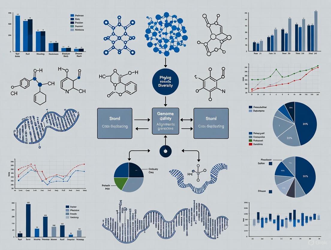
Resolving Phylogenetic Diversity in Cross-Species Genome Alignments: Methods, Challenges, and Clinical Applications

Abstract

This article provides a comprehensive overview of the computational and methodological landscape for resolving phylogenetic diversity from cross-species genome alignments, tailored for researchers and drug development professionals. It explores the foundational concepts of phylogenetic diversity metrics and their significance in biodiversity and biomedical research. The content delves into cutting-edge methodological advances, including the integration of deep learning, novel alignment tools, and phylogenetic networks for detecting evolutionary relationships and gene flow. It further addresses critical challenges in troubleshooting and optimizing large-scale phylogenetic analyses, covering issues from model misspecification to computational bottlenecks. Finally, the article offers a framework for the validation and comparative assessment of phylogenetic diversity, emphasizing robust statistical comparisons and the selection of appropriate metrics for conservation and trait discovery. This synthesis aims to bridge the gap between theoretical phylogenetics and its practical applications in identifying evolutionarily significant, functionally diverse genomic elements for biomedical innovation.

The Foundations of Phylogenetic Diversity: From Concepts to Genomic Data

Foundational Concepts and Definitions

What is Phylogenetic Diversity (PD)?

Phylogenetic Diversity (PD) is a measure of biodiversity that incorporates the evolutionary relationships between species. It is quantitatively defined as the sum of the lengths of all the branches on a phylogenetic tree that span the members of a set of species [1] [2]. This approach recognizes that not all species are equally distinct; some represent vastly more unique evolutionary history than others.

How does PD differ from simple species richness?

Unlike simple species counts, PD accounts for the phylogenetic difference between organisms. Two communities might have the same number of species, but the community containing species from more distantly related lineages will have a higher PD, capturing a greater amount of evolutionary history and, by inference, a greater variety of biological features [1] [3].

What is the core rationale for using PD in conservation and research?

The core rationale is that PD represents "feature diversity" and "option value." The branches in a phylogenetic tree represent the accumulation of evolutionary features (genetic, phenotypic, behavioral). Therefore, maximizing the PD preserved in a set of species also maximizes the preserved feature diversity, which maintains future benefits and options for humanity, such as new medicines or resilient crop traits [2].

A Framework for Phylogenetic Metrics

With over 70 different phylogenetic metrics in use, selecting the right one is critical. A unifying framework classifies these metrics into three primary dimensions based on their mathematical form and the ecological question they address [3].

The Three Dimensions of Phylogenetic Diversity

Dimension	Core Question	Representative Metric(s)	Typical Application
Richness	How much evolutionary history is represented?	Faith's PD (PD)	Conservation prioritization to maximize total evolutionary history preserved [1] [3].
Divergence	How different are the species from one another?	Mean Pairwise Distance (MPD)	Inferring community assembly processes (e.g., environmental filtering vs. competition) [3].
Regularity	How regular are the phylogenetic distances?	Variation of Pairwise Distance (VPD)	Understanding the evenness of evolutionary relationships within a community [3].

Diagram 1: A decision workflow for selecting phylogenetic diversity metrics based on research questions.

Troubleshooting Common Phylogenetic Analysis Problems

Why did my phylogenetic tree structure change drastically when I added more strains/species?

A sudden and drastic change in tree topology after adding new data can be caused by several factors [4]:

• Low sequence coverage in new strains: This leads to a higher number of ignored positions in the alignment, effectively reducing the informative core genome used for tree building.
• Presence of a severe outlier: A highly divergent or contaminated sample can distort the entire tree. Check for strains with an unusually high number of variants.
• Inappropriate handling of missing data: Some tree-building algorithms ignore positions not present in all samples. Using a method like RAxML, which can incorporate these positions, can restore the correct structure [4].
• Data concatenation errors: In one case, concatenating divergent sample replicates created artificial heterozygous positions that were ignored, collapsing diverse strains into a single branch. Removing these concatenated samples resolved the issue [4].

How can I assess the reliability of my phylogenetic tree?

Always check bootstrap values. These values test whether your entire dataset supports the tree structure. A common rule of thumb is that bootstrap values below 0.8 (or 80%) are considered weak [4]. Nodes with low support should not be trusted for biological interpretation.

My tree and my SNP-based clustering give conflicting signals. Which one is correct?

This conflict often arises because phylogenetic trees are typically built from a core genome alignment, while SNP-based clustering (like a "SNP address") can be generated from a full pairwise comparison of genomes [4]. If two strains look similar on the tree but are in different SNP clusters, it may indicate similarity in the core genome but divergence in accessory genes. Investigate the alignment method and the genomic regions used for each analysis.

Advanced Considerations: Phylogenetic Networks

When should I use a phylogenetic network instead of a tree?

Use a phylogenetic network when you have evidence or suspicion of reticulate evolutionary events, such as hybridization, introgression, or horizontal gene transfer, which cannot be represented by a strictly branching tree [5]. Networks are essential for studying groups where these processes are common.

How do I interpret a phylogenetic network?

In a rooted phylogenetic network, a reticulation vertex (a node with two incoming branches) represents a hybridization event [5]. The inheritance probability (γ), a value between 0 and 1 assigned to one of the incoming edges, denotes the proportion of genetic material the hybrid inherited from that parent. A value of γ ≈ 0.5 suggests symmetrical contributions from both parents [5].

Diagram 2: A phylogenetic network showing hybridization and introgression events with inheritance probabilities.

Essential Research Reagents and Tools

Key Software and Packages for Phylogenetic Diversity Analysis

Tool / Reagent	Function	Use Case
RAxML	Phylogenetic tree inference	Building large, accurate trees from molecular data; can handle positions not present in all samples [4].
FastTree	Phylogenetic tree inference	Rapid construction of approximate trees for large datasets [4].
CIPRES Cluster	Online computing platform	Provides free access to supercomputing resources for running compute-intensive analyses like RAxML [4].
V.PhyloMaker (R package)	Phylogeny generation	Constructing a phylogeny for a list of species using a broadly inclusive backbone (e.g., for vascular plants) [6].
picante / vegan (R packages)	Metric calculation	Calculating a wide array of phylogenetic diversity metrics within ecological communities [6].
EDGE of Existence program	Conservation prioritization	A global conservation initiative that uses evolutionary distinctness (a PD-related metric) to set priorities [1] [2].

For researchers in cross-species genome alignments, quantifying biodiversity extends beyond simple species counts. Phylogenetic diversity metrics leverage evolutionary relationships to provide a deeper understanding of genomic divergence and feature diversity. This guide details the core phylogenetic metrics—PDFaith, MPD, MNTD, NRI, and NTI—to assist in the selection, calculation, and interpretation of these measures in genomic studies [7] [3].

Frequently Asked Questions (FAQs)

1. What is the fundamental difference between PDFaith, MPD, and MNTD?

PDFaith, MPD, and MNTD capture different dimensions of evolutionary history. PDFaith (Faith's Phylogenetic Diversity) represents the total amount of evolutionary history in an assemblage by summing the branch lengths of the phylogenetic tree connecting a set of species [7]. MPD (Mean Pairwise Distance) measures the average evolutionary distance between all pairs of species in a sample, reflecting relatedness deep in the tree [7]. MNTD (Mean Nearest Taxon Distance) is the average evolutionary distance between each species and its closest relative in the sample, reflecting relatedness near the branch tips [7].

2. How do NRI and NTI help me infer ecological or evolutionary processes from my genomic data?

NRI (Net Relatedness Index) and NTI (Nearest Taxon Index) are standardized effect sizes that compare observed MPD and MNTD to values expected under a null model (e.g., a random assemblage from a regional species pool) [7].

• NRI is based on MPD. A significantly positive NRI indicates phylogenetic clustering (species are more closely related than expected by chance), which can suggest the influence of habitat filtering or limited dispersal. A significantly negative NRI indicates phylogenetic overdispersion (species are more distantly related than expected), which can suggest the influence of competitive exclusion [7].
• NTI is based on MNTD. It is often more sensitive to recent evolutionary events. The same interpretation for positive (clustering) and negative (overdispersion) values applies [7].

3. My analysis shows high species richness but low phylogenetic diversity (PDFaith). What does this imply for my study of cross-species genome alignments?

This result often indicates the presence of a recent, rapid radiation. The species in your assemblage are numerous but genetically very similar, having diverged from a common ancestor in a relatively short evolutionary time frame. For genome alignment research, this suggests that you are working with a clade of closely related species or lineages, where identifying genomic variations might require focusing on more rapidly evolving regions of the genome [7].

4. When should I use MPD versus MNTD to describe my genomic samples?

The choice depends on the scale of evolutionary history you wish to emphasize.

• Use MPD to understand deep evolutionary relationships and processes that have acted over long time scales. It provides a broad, "tree-wide" perspective on relatedness [7].
• Use MNTD to understand recent evolutionary relationships and processes, such as recent radiations or recent immigration events. It is more sensitive to patterns at the tips of the phylogenetic tree [7].

5. My phylogenetic tree is built from whole-genome alignments. Are there any special considerations for calculating these metrics?

High-throughput sequencing data, like whole-genome alignments, generally produce more robust and better-supported phylogenies compared to those built from a few genetic markers [7]. This strengthens the reliability of your PD metric calculations. Ensure that your branch lengths are proportional to the actual amount of genetic divergence (e.g., substitutions per site) as inferred from your alignments, as this is the fundamental input for all these metrics.

Troubleshooting Guide

Problem	Possible Cause	Solution
Unexpectedly low PDFaith	The assemblage may consist of many recently diverged species (a "bushy" clade) with short branch lengths [7].	Verify the phylogenetic tree topology. Check if the species set is monophyletic and has undergone a recent radiation. Consider if this aligns with the biological context.
NRI/NTI values are not significant	The phylogenetic structure of your assemblage does not significantly differ from a random draw from the species pool. The null model used may be inappropriate [7].	Review the composition of your regional species pool. Ensure the null model (e.g., random shuffling of tip labels) is appropriate for your research question and data.
MPD is high, but MNTD is low	The assemblage contains distinct, recent evolutionary radiations. Deep relationships are distant (high MPD), but within each deep branch, species are closely related (low MNTD) [7].	Investigate the tree for the presence of multiple closely-related clades that are distantly related to each other. This pattern is common in adaptive radiations.
Discrepancy between PD metrics and species richness	Rapid radiations, imbalanced phylogenies, or rare dispersal events can decouple species counts from evolutionary history [7].	This is an expected finding in many systems. Prioritize PD metrics if the goal is to capture feature diversity or evolutionary history, not just the number of taxa.
Poorly supported phylogenetic tree	The tree may be inferred from too few genetic markers, leading to unresolved relationships or unreliable branch lengths [7].	Use phylogenetic trees estimated from many genetic markers or whole-genome data for more reliable and well-supported results, which are critical for accurate PD calculations [7].

The table below provides a structured comparison of the core phylogenetic diversity metrics for easy reference [7].

Metric	Full Name	Interpretation	Calculation Basis	Standardized Metric
PDFaith	Faith's Phylogenetic Diversity	Total evolutionary history; higher values = greater diversity [7].	Sum of all branch lengths in the connecting tree [7].	PDSES
MPD	Mean Pairwise Distance	Average relatedness between all species pairs; higher values = more distantly related species (deep tree structure) [7].	Mean of all pairwise phylogenetic distances [7].	NRI (Net Relatedness Index)
MNTD	Mean Nearest Taxon Distance	Average relatedness to closest relative; lower values = more compact topology at tips [7].	Mean distance of each species to its nearest neighbor [7].	NTI (Nearest Taxon Index)
NRI	Net Relatedness Index	Phylogenetic structure vs. null model; + values = clustering, - values = overdispersion [7].	Standardized effect size of MPD [7].	---
NTI	Nearest Taxon Index	Phylogenetic structure at tips vs. null model; + values = clustering, - values = overdispersion [7].	Standardized effect size of MNTD [7].	---

Experimental Protocol: Calculating Phylogenetic Metrics from a Genome Alignment

This protocol outlines the key steps for deriving and interpreting phylogenetic diversity metrics from cross-species genome alignment data.

I. Materials and Software Requirements

• Input Data: Multi-sequence whole-genome alignment file (e.g., in FASTA, MAF, or VCF format).
• Computational Resources: High-performance computing (HPC) cluster or workstation with sufficient memory and CPU cores.
• Key Software Packages:
  • Phylogenetic Inference: IQ-TREE, RAxML, BEAST2.
  • Metric Calculation: R with packages picante, ape, PhyloMeasures.
  • Pipeline Integration: PhyloNext (for integrated data processing and analysis) [8].

II. Step-by-Step Procedure

• Phylogenetic Tree Inference:

  • Use your whole-genome alignment as input for a phylogenetic inference tool (e.g., IQ-TREE).
  • Select an appropriate nucleotide substitution model (e.g., ModelFinder within IQ-TREE).
  • Execute the analysis to generate a rooted, time-calibrated phylogenetic tree with branch lengths proportional to genetic divergence (substitutions/site). Save the output as a Newick file (.treefile).

• Assemblage Data Preparation:

  • Define the species assemblages for comparison (e.g., by geographic location, phenotypic group).
  • Create a community data matrix (presence/absence or abundance) in a format compatible with R, such as a comma-separated values (CSV) file.

• Metric Calculation in R:

  • Import the phylogenetic tree and community data into R.
  • Use the picante package to calculate the core metrics. Below is example R code for a single assemblage:

  • Note: The negative sign in the NRI/NTI calculation aligns with the convention that positive values indicate clustering [7].

• Interpretation and Visualization:

  • Compare metric values across your defined assemblages.
  • Statistically test the significance of NRI and NTI values against the null distribution.
  • Visualize results by plotting phylogenetic trees and highlighting assemblages of interest.

Workflow Visualization

The following diagram illustrates the logical workflow for deriving phylogenetic diversity metrics from genomic data.

Research Reagent Solutions

The table below lists key resources and tools essential for conducting phylogenetic diversity analysis in the context of genomic research.

Item Name	Category	Function in Analysis
IQ-TREE	Software	Efficient software for maximum likelihood phylogenetic inference from molecular sequences; supports a wide range of evolutionary models [8].
BEAST2	Software	Bayesian statistical software for phylogenetic analysis; used for inferring time-calibrated trees and complex evolutionary models.
R with picante package	Software / Library	The primary environment for calculating and analyzing phylogenetic diversity metrics, including PD, MPD, MNTD, NRI, and NTI [7].
Open Tree of Life (OToL)	Data Resource	Provides a comprehensive, synthetic phylogenetic tree of life, which can be used as a backbone or reference tree for analyses [8].
Global Biodiversity Information Facility (GBIF)	Data Resource	Provides standardized species occurrence data, which is used to define species assemblages for analysis [8].
PhyloNext Pipeline	Workflow Tool	An integrated computational pipeline (using Nextflow and Biodiverse) that streamlines the process from fetching GBIF data and OToL trees to calculating PD metrics [8].

Why Genome Alignments are Crucial for Accurate Phylogenetic Inference

Troubleshooting Guides

Guide 1: Resolving Alignment Artifacts and Frameshifts in Phylogenomic Analysis

Problem: Apparent frameshift mutations and shifted alignments in output, not representative of genuine biological mutations.

Explanation: Apparent frameshifts can result from local alignment errors rather than biological reality. These artifacts may be caused by low-quality sequencing data, inappropriate alignment parameters, or using evolutionarily distant reference species. Even sophisticated alignment pipelines can retain these errors, which subsequently bias phylogenetic inference and selection analyses [9] [10].

Solution:

• Implement comprehensive quality control: Run quality assurance on original reads using tools like FastQC and MultiQC before alignment [9].
• Filter alignment outputs: Remove low-quality alignments by keeping only primary alignments, proper pairs, or alignments with mapQ ≥ 20-30 [9].
• Apply post-alignment processing: Use BamLeftAlign to normalize alignments and Mark Duplicates to remove PCR artifacts [9].
• Verify reference consistency: Ensure the same reference genome assembly is used throughout analysis and visualization steps [9].
• Employ error-aware models: Use methods like BUSTED-E that incorporate an "error-sink" component to capture aberrant evolutionary patterns from alignment errors [10].

Prevention: For cross-species alignments, select reference genomes from species at appropriate evolutionary distances. Closer references (e.g., chimpanzee for human studies) help identify recent genomic events, while distant comparisons (e.g., human-pufferfish) primarily reveal coding sequences [11].

Guide 2: Addressing False Positive Selection Inference Due to Alignment Errors

Problem: Spuriously high rates of episodic diversifying selection (EDS) detected in genome-wide scans.

Explanation: Positive selection inference methods are highly sensitive to alignment errors. Even low error rates can profoundly bias EDS detection, as alignment errors can mimic patterns of positive selection. This problem often worsens with larger datasets as the probability of local alignment errors increases [10].

Solution:

• Apply BUSTED-E analysis: This method adds an error category (ωₑ ≥ 100) with maximum 1% weight to capture false signals from local alignment errors [10].
• Compare results with standard methods: Run both BUSTED and BUSTED-E analyses - a dramatic reversal in EDS support (e.g., p-value changing from 0.006 to 0.50) indicates likely alignment artifacts [10].
• Manual alignment inspection: Check regions with strong selection signals for local misalignment, particularly near sequence ends where errors often cluster [10].
• Use PRANK-C alignments: When computationally feasible, PRANK-C codon alignments are least affected by alignment errors and cannot be substantially improved by standard filtering programs [10].

Expected Outcome: BUSTED-E typically identifies pervasive residual alignment errors missed by automated filtering, produces more realistic positive selection estimates, reduces bias, and improves biological interpretation [10].

Guide 3: Optimizing Cross-Species Genome Alignment for Phylogenetic Diversity Assessment

Problem: Inadequate variant detection and phylogenetic resolution when using reference genomes from distantly related species.

Explanation: The evolutionary distance between target species and reference genome significantly impacts alignment completeness and variant detection. While felid species show high synteny conservation enabling successful cross-species alignment, more distant taxa may yield poor results [12].

Solution:

• Assess synteny conservation: For non-model species, first determine if a well-annotated reference from a related species exists with demonstrated synteny conservation [12].
• Validate with coverage metrics: Ensure >90% of reference genome is covered at sufficient depth (≥20x). Cheetah alignments to domestic cat reference achieved 94% properly paired reads, enabling discovery of 38+ million variants [12].
• Utilize multiple reference options: Test references at different evolutionary distances when possible. Read2Tree maintains higher precision with closer references but functions even with very distant references [13].
• Consider alignment-free methods: For extremely distant comparisons, tools like Read2Tree can process raw reads directly into orthologous groups, bypassing genome assembly and traditional alignment [13].

Performance Metrics: Successful cross-species alignments should achieve >90% reference coverage with proper pairing, enabling comprehensive variant discovery comparable to within-species alignments [12].

Frequently Asked Questions

Q1: What are the key considerations when selecting reference species for cross-species genome alignments?

A: Reference selection depends on your biological question. For identifying functional elements, use species at intermediate evolutionary distances (diverged 40-80 million years) like human-mouse comparisons, which reveal both coding and conserved noncoding sequences. For primarily detecting coding sequences, use distantly related species (diverged ~450 million years). To identify recent evolutionary changes, use closely related species [11].

Q2: How do alignment errors specifically affect phylogenetic inference and selection analyses?

A: Alignment errors create false phylogenetic signals that mimic biological patterns. They increase false positive rates in diversifying selection tests, distort branch lengths, and can lead to incorrect tree topologies. Methods like BUSTED-E show that many genes initially flagged under positive selection are actually explained by alignment errors [10].

Q3: What computational strategies can handle large-scale phylogenomic datasets with hundreds of species?

A: New tools address scalability challenges: Phyling uses profile-based ortholog identification rather than all-against-all searches, enabling incremental dataset updates without reprocessing [14]. Read2Tree bypasses genome assembly entirely, processing raw reads directly into orthologous groups, achieving 10-100x speedup over assembly-based approaches while maintaining accuracy [13].

Q4: How reliable are cross-species alignments for variant discovery in non-model organisms?

A: When synteny is high, cross-species alignment works remarkably well. Felid studies aligned cheetah, snow leopard and Sumatran tiger to domestic cat reference, achieving 93-95% properly paired reads and discovering millions of high-quality variants. However, this approach has limitations in detecting rare variants [12].

Table 1: Impact of Evolutionary Distance on Alignment Detection Sensitivity

Comparison Type	Divergence Time	Primary Sequences Detected	Utility
Closely Related (e.g., Human-Chimpanzee)	~7 million years	Recent genomic changes, species-specific sequences	Identifying traits unique to reference species
Intermediate Distance (e.g., Human-Mouse)	40-80 million years	Coding sequences + conserved noncoding sequences	Finding functional noncoding elements
Distantly Related (e.g., Human-Pufferfish)	~450 million years	Primarily coding sequences	Gene identification and annotation

Table 2: Performance Benchmarks of Alignment and Phylogenetic Tools

Tool	Methodology	Advantages	Limitations
Phyling	Profile-based ortholog identification using HMM profiles from BUSCO	Fast, scalable to thousands of species; checkpoint system for incremental updates	Lower accuracy with very distant references [14]
Read2Tree	Direct raw read processing into orthologous groups	10-100x faster than assembly-based approaches; works with low-coverage (0.1×) data	Slightly lower accuracy with high coverage and very distant references [13]
BUSTED-E	Branch-site random effects model with error-sink component	Identifies residual alignment errors; reduces false positive selection inference	Requires reasonable alignment quality to start [10]

Experimental Protocols

Protocol 1: Cross-Species Variant Discovery Using Divergent Reference Genomes

Purpose: To identify single nucleotide variants (SNVs) in non-model species using reference genomes from related species.

Materials:

• Whole genome sequencing data from target non-model species
• High-quality reference genome assembly from related model species
• Computing infrastructure with ≥16GB RAM
• BWA-MEM2 or similar aligner [9]
• GATK or similar variant calling toolkit [12]

Methodology:

• Quality Control: Assess raw read quality using FastQC and MultiQC.
• Alignment: Map reads to reference genome using BWA-MEM2 with species-appropriate parameters.
• Processing: Convert, sort, and index alignment files; remove PCR duplicates.
• Variant Calling: Identify SNVs using HaplotypeCaller in GATK.
• Filtering: Apply variant quality score recalibration and hard filters.
• Annotation: Annotate variants using VEP or SnpEff with available gene models.

Validation: Expect >90% reference genome coverage with proper pairing. For felid species, cheetah alignments to domestic cat achieved 94% properly paired reads, enabling discovery of 38,839,061 variants [12].

Protocol 2: Phylogenomic Tree Inference with Error-Aware Selection Analysis

Purpose: To infer species phylogenies while accounting for alignment errors that bias selection inference.

Materials:

• Multiple sequence alignments of orthologous genes
• Phylogenetic tree inference software (IQ-TREE, RAxML-NG, or FastTree)
• HyPhy package with BUSTED and BUSTED-E methods [10]
• Computational resources for likelihood calculations

Methodology:

• Ortholog Identification: Extract orthologous sequences using Phyling (profile-based) or OrthoFinder (RBH-based) approaches [14].
• Alignment: Create multiple sequence alignments using MAFFT or PRANK-C.
• Tree Inference: Construct initial phylogenies using maximum likelihood or concatenation approaches.
• Selection Analysis:
  • Run standard BUSTED analysis to test for episodic diversifying selection
  • Run BUSTED-E analysis with error-sink component (ωₑ ≥ 100, max 1% weight)
  • Compare results: dramatic changes in significance indicate alignment error contamination
• Visualization: Inspect alignment regions flagged by BUSTED-E for manual verification.

Interpretation: BUSTED-E typically reduces false positive selection calls. In one analysis, UROD gene significance dropped from p=0.006 (BUSTED) to p=0.50 (BUSTED-E), with selection signal absorbed by error class [10].

Workflow Visualization

Title: How Alignment Errors Impact Phylogenetic Inference and Mitigation Strategies

Research Reagent Solutions

Table 3: Essential Bioinformatics Tools for Phylogenomic Analysis

Tool/Category	Specific Examples	Primary Function	Application Notes
Alignment Tools	BWA-MEM2, PRANK-C	Map reads to reference genomes	PRANK-C particularly robust for selection analysis [10]
Orthology Inference	Phyling, OrthoFinder	Identify orthologous genes across species	Phyling uses profile-based approach for scalability [14]
Variant Callers	GATK, SAMtools	Identify genetic variants from alignments	Critical for cross-species comparisons [12]
Selection Analysis	BUSTED-E, PAML	Detect positive selection	BUSTED-E incorporates error modeling [10]
Tree Inference	IQ-TREE, RAxML-NG, ASTRAL	Phylogenetic tree construction	Concatenation vs. consensus approaches available [14]
Error Detection	BUSTED-E, manual inspection	Identify alignment artifacts	Essential for reliable phylogenetic inference [10]

Linking Evolutionary History to Biodiversity and Trait Diversity

Frequently Asked Questions

FAQ 1: What are the primary considerations when selecting a reference genome for a cross-species alignment study? The key considerations are evolutionary distance and assembly quality. For closely related species, you can use a high-quality reference genome from a closely related organism due to high genomic synteny [12]. For more distantly related species, a high-quality, chromosome-level assembly from the best-studied species in the clade is preferable. Always prioritize assemblies with fewer gaps and high sequencing depth over draft-quality assemblies, as the latter can contain errors that bias biological conclusions [12].

FAQ 2: My cross-species alignment shows high coverage, but my variant calls have an unusually high number of putative deleterious mutations. What could be the cause? This pattern often indicates a problem with the reference genome or the alignment itself, but it can also be a true biological signal. First, ensure you are not using a draft-quality assembly with known errors [12]. If the reference is validated, this pattern could accurately reflect the population history of your study species. Low genetic diversity and a high burden of deleterious variants are genomic signatures of endangered species with recent population declines [15]. Compare your findings to the species' conservation status.

FAQ 3: How can I distinguish between functional non-coding sequences and neutrally evolving sequences in a multi-species alignment? The strategy involves comparing species at different evolutionary distances [11]. Sequences conserved between distantly related species (e.g., human and pufferfish, which diverged ~450 million years ago) are almost certainly under functional constraint and are often coding exons. Sequences conserved between moderately related species (e.g., human and mouse, diverged ~80 million years ago) can include both coding and functional non-coding elements, like regulatory regions. Adding a closely related species (e.g., human and chimpanzee) helps identify recently evolved sequences and species-specific traits [11].

FAQ 4: What is the difference between "conserved synteny" and a "conserved segment"? These terms describe different levels of conserved genome architecture. Conserved synteny means that groups of genes (orthologs) are located on the same chromosome in two different species, regardless of their order or orientation. A conserved segment (or conserved linkage) is a stricter definition; it means that the order of multiple orthologous genes is the same in the two species [11].

FAQ 5: Can I use a cross-species alignment to test adaptive versus non-adaptive evolutionary hypotheses? Yes, this is a primary application of comparative genomics. To test an adaptive hypothesis, you must first construct a null model. In evolution, a null model often explains a trait as arising through non-adaptive processes like mutation accumulation or genetic drift [16]. For example, the mutation accumulation (MA) model is a null hypothesis for aging, positing that deleterious mutations with late-acting effects persist because natural selection is too weak to remove them. To argue for adaptation, you must provide evidence that your observation (e.g., the rate of aging) is too pronounced to be explained by the null model alone [16].

---

Troubleshooting Guides

Issue 1: Poor Alignment Coverage and Mapping Rates

• Problem: A low percentage of your sequencing reads are successfully mapping to the reference genome.
• Solution:
  • Verify Reference Genome Quality: Check the assembly quality of your reference genome. Prefer chromosome-level builds (like felCat9 for felids [12]) over fragmented draft assemblies.
  • Check for Contamination: Ensure your DNA sample is not contaminated with foreign DNA.
  • Assess Evolutionary Distance: The reference species may be too evolutionarily distant from your study species. Try a reference genome from a closer relative. High mapping rates (>90%) are achievable when aligning big cat genomes to the domestic cat reference, demonstrating the utility of this approach within families [12].
  • Inspect Raw Read Quality: Use tools like FastQC to check for adapter contamination or poor sequencing quality.

Issue 2: Inability to Delineate Population Structure

• Problem: Variant data from cross-species alignment fails to reveal expected population structure.
• Solution:
  • Increase Sample Size: The power to detect population structure increases with the number of individuals sequenced.
  • Switch from Pooled to Individual Sequencing: Non-barcoded pooled sequencing (PoolSeq) can be limited in its ability to detect rare variants and delineate fine-scale population structure. Transitioning to individual whole-genome sequencing provides genotype data for each individual, which is superior for population analysis [12].
  • Filter Variants Rigorously: Apply strict quality filters to your variant calls (SNVs) to minimize false positives that can obscure biological signals.

Issue 3: High Heterozygosity Complicating Genome Assembly

• Problem: Difficulty in achieving a contiguous genome assembly for a species, often correlated with high heterozygosity [15].
• Solution:
  • Use Specialized Assemblers: Employ assembly algorithms designed for highly heterozygous genomes.
  • Utilize Long-Read Technologies: Sequence using long-read technologies (e.g., PacBio, Oxford Nanopore) to span repetitive and heterozygous regions.
  • Employ Proximity Ligation: Techniques like Hi-C can scaffold a fragmented assembly into chromosome-length scaffolds, dramatically improving contiguity, even for challenging genomes [15].

---

Data Presentation

Table 1: Exemplar Alignment and Variant Call Metrics from a Cross-Species Study in Felids [12]

This table summarizes key quantitative outcomes from a study that aligned three big cat species to the domestic cat (Felis catus) reference genome (felCat9), providing a benchmark for expected results.

Species	Read Pairs Mapped (Millions)	Properly Paired & Mapped	Biallelic SNVs Called	Transitions (Ts)	Transversions (Tv)
Cheetah (Acinonyx jubatus)	170 (avg.)	94%	38,839,061	26,430,702	12,408,359
Snow Leopard (Panthera uncia)	627 (avg.)	93%	15,504,143	9,124,699	4,285,891
Sumatran Tiger (Panthera tigris sumatrae)	251 (avg.)	95%	13,414,953	10,472,528	5,030,622

Table 2: Genetic Diversity Metrics from the Zoonomia Project for Conservation Prioritization [15]

This table illustrates how reference genome metrics from a single individual can inform conservation status. SoH (Segments of Homozygosity) is a robust metric less affected by assembly contiguity.

Species / Grouping	Metric	Value / Correlation	Conservation Insight
126 DISCOVAR Assemblies	Correlation (Overall Heterozygosity vs. SoH)	Pearson's r = -0.56	Confirms that lower diversity is linked to more homozygous stretches.
Giant Otter (Pteronura brasiliensis)	Low diversity & high deleterious variants	Found	Consistent with known population decline; has higher recovery potential than sea otters [15].
General Finding	Heterozygosity in threatened species	Generally lower	A genome from a single individual can help identify at-risk populations [15].

---

Experimental Protocols

Protocol 1: Cross-Species SNV Discovery Using a Reference Genome

This methodology is adapted from a study that successfully identified single nucleotide variants in big cats by aligning to the domestic cat genome [12].

• DNA Source: Obtain high-quality genomic DNA from the target non-model species. DNA can be from tissue, blood, or cell cultures. The Frozen Zoo at San Diego Zoo Global is a key resource for endangered species [15].
• Sequencing: Perform whole-genome sequencing on an Illumina platform. For individual samples, aim for a minimum coverage of 10-15x. For non-barcoded pooled sequencing (PoolSeq), pool DNA from multiple individuals in equimolar ratios and sequence to a higher depth (e.g., >25x) to ensure coverage of rare alleles [12].
• Alignment: Map the sequenced reads to a high-quality reference genome (e.g., felCat9 for felids) using a standard aligner like BWA-MEM.
• Variant Calling: Call biallelic single nucleotide variants (SNVs) in diploid mode for all samples using a caller like GATK HaplotypeCaller or SAMtools/bcftools.
• Variant Annotation and Filtering: Annotate variants using a tool like SnpEff and the reference genome's annotation. Apply quality filters (e.g., on depth, quality score, and mapping quality) to generate a high-confidence set of variants.
• Downstream Analysis: Use the filtered SNVs for population structure analysis (e.g., with ADMIXTURE), calculating nucleotide diversity (π), and enrichment analysis of fixed and species-specific SNVs.

Protocol 2: Assessing Phylogenetic Diversity and Evolutionary Constraint with a Multi-Species Alignment

This protocol is based on the design and implementation of large-scale comparative genomics projects like Zoonomia [15].

• Species Selection: Maximize evolutionary branch length by selecting at least one species from each family within the clade of interest. Prioritize species of medical, biological, or conservation concern.
• Genome Assembly & Curation: Generate genome assemblies using a consistent method (e.g., DISCOVAR de novo for short-read contigs [15]) to minimize technical variation. For a subset, perform proximity ligation (Hi-C) to create chromosome-level scaffolds.
• Whole-Genome Alignment: Use a specialized pipeline (e.g., CACTUS) to create a multiple whole-genome alignment of all selected species, independent of a single reference genome.
• Measuring Constraint: Identify evolutionarily constrained regions by detecting nucleotides that have remained unchanged across millions of years of evolution more than expected by chance alone. This is powerful for annotating functional genomes [15].
• Linking to Traits: Overlap species-specific genetic changes (e.g., accelerated evolution, conserved non-coding elements) with phenotypic data to generate hypotheses about the genetic basis of traits like venom production or cancer resistance [15].

---

Mandatory Visualization

Diagram 1: Cross-Species Variant Discovery Workflow

Diagram 2: Evolutionary Hypothesis Testing Logic

---

The Scientist's Toolkit

Table 3: Essential Research Reagents and Resources

Item	Function / Description
High-Quality Reference Genome	A chromosome-level assembly of a closely related or model species used for read alignment and variant discovery. Essential for providing genomic context [12].
The Frozen Zoo (San Diego Zoo Wildlife Alliance)	A biorepository storing renewable cell cultures from over 1,100 taxa, including many endangered species. A critical source of DNA for non-model organism genomics [15].
Whole-Genome Alignment (WGA)	A multitool for scientific discovery. Enables the identification of evolutionarily constrained regions and species-specific changes by comparing multiple genomes simultaneously [15].
Orthologous Sequences	Genes in different species that evolved from a common ancestral gene by speciation. Comparisons between orthologs are critical for identifying functional elements [11].
Paralogous Sequences	Genes related by duplication within a genome. Comparisons between paralogs are more divergent and less informative for cross-species functional analysis than orthologs [11].

The Limitation of Traditional Statistics and the Rise of Phylogenetic Comparisons

Frequently Asked Questions (FAQs)

FAQ 1: What are the main limitations of traditional statistical methods in genomic analysis? Traditional statistics often assume that data points are independent and identically distributed. However, in cross-species genomic studies, species are related through an evolutionary tree, violating this core assumption. This can lead to:

• Increased False Positives: Failure to account for shared evolutionary history (phylogenetic non-independence) can inflate Type I errors, mistakenly identifying patterns as significant.
• Oversimplified Models: Traditional methods struggle to model complex evolutionary processes like gene flow, hybridization, and incomplete lineage sorting, which are common in genomic datasets [5].
• Inaccurate Conclusions: Without a phylogenetic framework, it is easy to misinterpret shared genetic similarities as evidence of direct relationship or recent function, when they may be due to ancestral traits or convergent evolution [17].

FAQ 2: How do phylogenetic comparisons address the problem of non-independence? Phylogenetic comparative methods explicitly incorporate the evolutionary relationships among species into the statistical model. By using a phylogenetic tree, these methods:

• Model Covariance: They treat species as related tips on a tree, with their expected covariance based on shared branch lengths.
• Distinguish Homology from Homoplasy: They help differentiate between similarities due to common descent (homology) and those arising independently (homoplasy or convergent evolution) [17].
• Provide an Evolutionary Framework: This allows researchers to test hypotheses about trait evolution, selection, and adaptation in a statistically robust manner.

FAQ 3: What is the difference between a phylogenetic tree and a phylogenetic network, and when should I use a network? You should use a phylogenetic network when your data shows strong, conflicting signals that cannot be explained by a simple tree-like evolutionary history [5].

Feature	Phylogenetic Tree	Phylogenetic Network
Underlying Model	Assumes strictly divergent, tree-like evolution.	Generalizes trees to incorporate reticulate events like hybridization and gene flow.
Visual Structure	Strictly branching (bifurcating).	Includes both branches and reticulations (nodes with two incoming edges).
Best Used For	Scenarios where vertical descent is the primary evolutionary process.	Scenarios involving hybridization, horizontal gene transfer, or hybrid speciation [5].

FAQ 4: My phylogenetic analysis shows conflicting signals. How can I determine if it's due to incomplete lineage sorting (ILS) or hybridization? Distinguishing between ILS and hybridization is a key challenge. You can approach it as follows:

• Use Specific Methods: Employ methods based on the Network Multi-Species Coalescent (NMSC), which are designed to model both ILS and hybridization simultaneously [5].
• Analyze Gene Tree Variation: Compare gene trees from across the genome. While both processes cause gene tree discordance, hybridization creates specific patterns that can be detected.
• Leverage Hybridization Tests: Use statistical tests like Patterson's D-statistic (ABBA-BABA test) to detect signals of gene flow between lineages. However, be aware that these tests can be sensitive to violations of assumptions and perform poorly with multiple or ghost reticulations [5].

FAQ 5: How can phylogenetic analysis be applied in drug discovery? Phylogenetic analysis is crucial for identifying and validating new drug targets [18].

• Target Identification: It helps pinpoint evolutionarily conserved regions in proteins (e.g., enzymes, receptors) that are crucial for function and can be targeted by drugs.
• Understanding Pathogen Evolution: By reconstructing the phylogenetic history of pathogens, researchers can track the emergence and spread of drug-resistant strains, informing drug and vaccine design [18].
• Natural Product Discovery: A correlation between phylogeny and biosynthetic pathways can predict which related plant species are likely to produce similar bioactive compounds, streamlining the selection of candidates for chemical analysis [17].

Troubleshooting Guides

Problem 1: Inconsistent or Weak Support for Phylogenetic Clades Potential Cause: The evolutionary model may be misspecified, or the data may contain conflicting signals from processes like Incomplete Lineage Sorting (ILS). Solution:

• Step 1 - Model Selection: Use model selection tools (e.g., in IQ-TREE) to find the best-fit nucleotide or amino acid substitution model for your data [18].
• Step 2 - Data Exploration: Consider partitioning your data (by gene, codon position) and analyzing partitions separately to identify conflicting signals.
• Step 3 - Method Upgrade: If ILS is suspected, switch to a method that explicitly models it, such as coalescent-based species tree methods (e.g., ASTRAL) or phylogenetic network methods (e.g., SNaQ) that account for both ILS and hybridization [5].

Problem 2: Detecting Reticulate Evolution but Unclear Interpretation Potential Cause: Challenges in biologically interpreting the inferred phylogenetic network, particularly the direction of gene flow or the nature of the hybridization event. Solution:

• Step 1 - Understand Reticulation Parameters: In a network, a reticulation vertex has an inheritance probability (γ), which denotes the proportion of genetic material the hybrid lineage inherited from one parent. A value of 0.5 suggests symmetrical hybridization, while values close to 0 or 1 suggest asymmetrical introgression [5].
• Step 2 - Distinguish Event Types: Be cautious in interpretation. A γ of 0.5 could indicate an F1 hybrid species or repeated backcrossing with both parents. The method alone may not distinguish between recent and ancient events without additional biological evidence [5].
• Step 3 - Incorporate External Evidence: Use information from geography, morphology, or known reproductive biology to constrain and validate the plausible biological interpretations of the network.

Problem 3: Computational Limitations with Large Genomic Datasets Potential Cause: Phylogenetic analyses, especially Bayesian inference or large bootstrap analyses, are computationally intensive and time-consuming. Solution:

• Step 1 - Use Efficient Software: Opt for fast and memory-efficient programs like IQ-TREE for maximum likelihood analysis [18].
• Step 2 - Reduce Data Complexity: For initial exploration, use a subset of data (e.g., one representative per species) or a reduced set of informative sites.
• Step 3 - Leverage High-Performance Computing (HPC): Scale your analyses by utilizing HPC clusters or cloud computing resources.
• Step 4 - Explore Scalable Network Methods: Newer methods for inferring explicit phylogenetic networks are becoming more scalable and effective with hundreds of loci, making them applicable to typical phylogenomic datasets [5].

Experimental Protocols & Data

Protocol 1: Testing for Phylogenetic Signal in Chemical Traits This protocol is used to determine if the production of specific chemical compounds (e.g., alkaloids) is correlated with the evolutionary relationships among species [17].

• Sample Collection: Gather plant material from a taxonomically diverse set of species within a clade of interest (e.g., Amaryllidoideae).
• DNA Sequencing & Phylogeny Reconstruction: Sequence multiple DNA regions (e.g., ITS, matK) from all samples. Use parsimony and Bayesian inference to reconstruct a robust phylogenetic hypothesis [17].
• Chemical Profiling: Extract and analyze specialized metabolites from each species using Liquid Chromatography-Mass Spectrometry (LC-MS). Identify and quantify the diversity of compounds, such as different alkaloid types.
• Bioactivity Assay: Perform relevant bioassays (e.g., acetylcholinesterase (AChE) inhibition for Alzheimer's research) on the extracts [17].
• Statistical Analysis: Use comparative phylogenetic methods (e.g., Blomberg's K, Pagel's λ) to test whether chemical diversity and bioactivity show a significant phylogenetic signal.

Quantitative Data from a Model Study (Amaryllidoideae) [17] The table below summarizes the data sources and their contribution to a phylogenetic analysis, demonstrating the power of combined evidence.

DNA Region	Number of Aligned Characters	Potentially Parsimony-Informative Characters (%)	Key Outcome
ITS	953	502 (53%)	The most informative individual region.
Plastid Combined	3182	480 (15%)	Provided strong support for major lineages.
Total Evidence	5861	1086 (19%)	Resolved 87% of clades, the highest of any analysis.

Protocol 2: Phylogenetic Target Identification in Pathogens This methodology helps identify conserved and pathogen-specific proteins as potential drug targets [18].

• Genome Assembly: Collect or sequence genomes for multiple strains and species of a pathogen (e.g., Mycobacterium tuberculosis) and related non-pathogens.
• Gene Family Identification: Use orthology prediction tools to group genes into families across all genomes.
• Phylogenetic Profiling: For each gene family, reconstruct a phylogenetic tree to identify:
  • Genes that are conserved and essential in the pathogen.
  • Genes that are absent from the human host.
• Prioritization: Prioritize candidate targets that are conserved across the pathogen, present in a broad range of strains, and absent or highly divergent in the host to minimize off-target effects [18].

The Scientist's Toolkit: Research Reagent Solutions

Item	Function in Phylogenomic Analysis
IQ-TREE	A software for maximum likelihood phylogenomic inference. It incorporates model selection to find the best-fit evolutionary model, making phylogenetic inference more accurate and robust [18].
Patterson's D-Statistic	A hybridization test used to detect gene flow between lineages by analyzing patterns of allele sharing among four taxa. It is practical for identifying specific reticulate events [5].
Vega Visualization Grammar	A higher-level language for creating customizable, interactive visualizations. It is useful for generating complex phylogenetic trees and networks from JSON specs, aiding in data exploration and presentation [19].
Multi-Species Coalescent Model	A population genetics model that accounts for gene tree-species tree discordance caused by Incomplete Lineage Sorting (ILS). It is fundamental for delimiting species and analyzing traits from genomically diverse datasets [5].
Phylodynamic Modeling	A framework that combines phylogenetic data with epidemiological information. It is used to simulate and predict the spread of infectious diseases, informing the timely design of drug therapies and vaccines [18].

Workflow and Relationship Visualizations

Diagram 1: Traditional vs phylogenetic analysis workflow.

Diagram 2: Phylogenetic analysis for drug discovery.

Advanced Methods for Phylogenetic Inference from Genomic Data

Cross-species genome alignment is a foundational step in resolving phylogenetic diversity. It allows researchers to identify conserved functional elements, understand evolutionary constraints, and pinpoint rapidly changing genomic regions. For phylogenetic studies spanning divergent species, the choice of alignment tool is critical, as it must capture homologous sequences separated by vast evolutionary distances. The core challenge lies in balancing the exceptional sensitivity required to detect these distant homologies with the computational speed needed to process genome-scale data. Among the available tools, lastZ has been the long-standing benchmark for sensitivity, while its modern, GPU-accelerated derivative, KegAlign, promises to maintain this sensitivity at a fraction of the runtime [20] [21]. This technical support center addresses the specific issues researchers encounter when employing these tools in demanding cross-species phylogenetic projects.

---

Frequently Asked Questions (FAQs)

Q1: Why is lastZ often recommended for cross-species alignment over faster tools like minimap2?

A1: lastZ is renowned for its superior sensitivity when aligning evolutionarily divergent sequences. While tools like minimap2 are dramatically faster, lastZ excels at finding homologies between genomes that have undergone significant sequence change. Benchmarking tests show that lastZ consistently generates end-to-end alignments across a wide range of sequence divergence (from 0% to 40%), and its alignments cover the vast majority of protein-coding exons in comparisons between species as distant as human and mouse [20] [21]. This sensitivity is crucial for phylogenetic studies that include deeply divergent taxa.

Q2: What is the primary performance bottleneck when running lastZ on large genomes?

A2: The main bottleneck is the immense computational time required. A standard mammalian whole-genome alignment using lastZ can take approximately 2,700 CPU hours. Scaling this to align 100 vertebrate genomes with a human reference would take an estimated 30 CPU years, making lastZ the primary obstacle for large-scale phylogenetic alignment projects [20] [21].

Q3: How does KegAlign address the speed limitations of lastZ?

A3: KegAlign is a GPU-enabled refactoring of the lastZ algorithm. It introduces a novel diagonal partitioning parallelization strategy and leverages advanced NVIDIA GPU features like Multi-Instance GPU (MIG) and Multi-Process Service (MPS). This optimization allows KegAlign to compute a human-mouse alignment in under 6 hours on a single node with an NVidia A100 GPU and 80 CPU cores, representing a speedup of approximately 150 times over lastZ without sacrificing sensitivity [20] [21].

Q4: What are the common hardware utilization problems with earlier GPU-accelerated aligners like SegAlign?

A4: SegAlign, a predecessor to KegAlign, suffered from severe hardware underutilization due to tail latency. The tool partitioned input sequences into equally-sized segments, which did not translate to equally-sized computational workloads. For closely related genomes (e.g., human-chimp), some segment pairs required vastly more time for gapped extension than others (up to 10,000 times longer than the median). This caused most CPU and GPU resources to sit idle while waiting for a few long-running tasks to complete, a problem that could not be solved by simply adding more hardware [20].

Q5: How should I choose alignment parameters for species at different evolutionary distances?

A5: Alignment strategy should be tailored to the evolutionary divergence of the species being compared. The following table summarizes recommended presets and tools for different scenarios [22]:

Evolutionary Distance	Example Species Pair	TimeTree (MYa)	Recommended Aligner	Suggested Preset
Same Species	Human (build 38) vs. Human (build 37)	0	BLAT, GSAlign	-tileSize=11 -minScore=100 -minIdentity=98 (BLAT)
Near / Primate	Human vs. Chimpanzee	6.7	lastZ / KegAlign	primate or E=30 H=3000 K=5000 L=5000 M=10 [22]
Medium / General	Human vs. Mouse	90	lastZ / KegAlign	general or E=30 H=3000 K=5000 L=5000 M=10 [22]
Far / Distant	Human vs. Chicken	312	lastZ / KegAlign	far or E=30 H=2000 K=2200 L=6000 M=50 O=400 T=2 [22]

---

Troubleshooting Guides

Problem 1: Extremely Long Runtime with lastZ

Symptoms: An alignment job is taking days or weeks to complete, severely hampering research progress.

Diagnosis and Solution:

Potential Cause	Diagnostic Steps	Recommended Solution
Large, divergent genomes	Check the sizes and estimated divergence of your input genomes.	Switch from lastZ to KegAlign to leverage GPU acceleration [20] [21].
Suboptimal sensitivity settings	Review the parameters. Using default, high-sensitivity settings on large sequences is computationally expensive.	For an initial survey, use a lower-sensitivity preset (e.g., --notransition --step=20). Reserve high-sensitivity runs for final analyses [23].
Inefficient sequence partitioning	The job is running on a single thread without any parallelization.	If KegAlign is not an option, partition the input sequences into smaller fragments (e.g., by chromosome or smaller chunks) and run lastZ jobs in parallel on a compute cluster [20].

Problem 2: Poor Alignment Sensitivity on Divergent Genomes

Symptoms: The resulting alignment fails to cover known functional elements (e.g., exons) when comparing distant species.

Diagnosis and Solution:

Potential Cause	Diagnostic Steps	Recommended Solution
Overly aggressive speed-optimized tools	The aligner used (e.g., minimap2) is optimized for speed, not deep divergence.	Use lastZ or KegAlign as the primary aligner, as they are specifically designed for sensitivity across evolutionary timescales [20] [21].
Incorrect scoring parameters	Check if the scoring matrix and parameters match the evolutionary distance.	Use evolutionarily-informed parameter presets. For distant species, use the "far" preset with parameters like H=2000 K=2200 L=6000 which are tuned for lower sequence similarity [22].
Algorithmic limitations	The tool uses a protein-level rather than nucleotide-level comparison, missing non-coding regions.	For aligning non-coding UTRs or other non-translated sequences, a nucleotide-level tool like lastZ/KegAlign is the only option [24].

Problem 3: Low Hardware Utilization with KegAlign/SegAlign

Symptoms: GPU and CPU usage metrics show significant idle time, despite a running job.

Diagnosis and Solution:

Potential Cause	Diagnostic Steps	Recommended Solution
CPU/GPU workload imbalance (Tail Latency)	Monitor per-core CPU usage. One or a few cores are at 100% while others are idle.	This was a key flaw in SegAlign. KegAlign's diagonal partitioning strategy is specifically designed to mitigate this by creating more balanced work units. Ensure you are using KegAlign, not SegAlign [20].
GPU data starvation	GPU utilization drops sharply after an initial period, while CPUs remain busy.	This is caused by back pressure from the gapped-extension stage. KegAlign's use of MPS (Multi-Process Service) helps optimize GPU workload scheduling and communication to reduce idle time [20] [21].

---

Experimental Protocols

Protocol 1: Benchmarking Alignment Sensitivity and Coverage

This protocol is used to evaluate how well an aligner recovers homologous regions between divergent genomes, such as in a phylogenetic context.

• Input Preparation: Create a set of "homologous" sequence pairs of varying lengths (e.g., 1kb, 2kb, 5kb, 10kb) with simulated divergence from 0% to 40% in 1% increments. Add random 1,000 nucleotide flanks to the 5' and 3' ends of each sequence [20] [21].
• Alignment Execution: Run the target aligners (e.g., lastZ, KegAlign, minimap2) on these sequence pairs using their recommended parameters for divergent sequences.
• Sensitivity Calculation: For each alignment output, calculate the alignment coverage, defined as the fraction of the original homologous sequence included in the final alignment block.
• Visualization and Analysis: Plot alignment coverage against sequence divergence and length. A sensitive aligner will maintain high coverage even at high divergence rates [20] [21].
• Validation with Biological Data: As a validation step, perform a whole-genome alignment (e.g., human vs. mouse) and compute the fraction of protein-coding exons from the reference genome that are covered by the alignments. Merge overlapping alignments and exons to eliminate redundancy before calculating coverage [20].

Protocol 2: Evaluating Runtime Performance and Hardware Utilization

This protocol assesses the computational efficiency of an aligner, which is critical for project planning on shared or limited resources.

• Baseline Establishment: Run a standard alignment task (e.g., human chromosome 1 vs. mouse chromosome 1) using a baseline tool like lastZ on a defined CPU-only system. Record the total wall-clock time and CPU time [20] [21].
• Test Execution: Run the same alignment task with the optimized tool (e.g., KegAlign) on a system with a capable GPU (e.g., containing an NVidia A100).
• Resource Monitoring: During the run, use system monitoring tools (e.g., nvtop for GPU, htop for CPU) to track:
  • GPU Utilization: The percentage of time the GPU is actively processing data.
  • CPU Utilization: The per-core and overall CPU usage.
  • Memory Usage: System and GPU memory consumption.
• Performance Analysis: Calculate the speedup as: Baseline Runtime (lastZ) / Optimized Runtime (KegAlign). Analyze monitoring logs to identify hardware underutilization, such as tail latency where most resources wait for a few slow tasks [20].
• Data Presentation: Summarize key performance metrics in a table for clear comparison.

Table: Example Performance Benchmark (Human chr1 vs. Mouse chr1) [21]

Tool	Hardware	Runtime	Relative Speed
lastZ	CPU	~208 minutes	1x (Baseline)
minimap2	CPU	~0.6 minutes	~347x faster
KegAlign	GPU (A100) + CPU	< 6 hours (full genome)	~150x faster than lastZ

---

Workflow Visualization

The following diagram illustrates the core alignment process optimized by KegAlign and lastZ, highlighting the critical stages and bottlenecks.

Diagram Title: Genome Alignment Core Workflow

---

The Scientist's Toolkit: Essential Research Reagents & Materials

Table: Key Software and Hardware for Genomic Alignment

Item Name	Function / Application	Notes for Phylogenetic Studies
lastZ	The sensitive, CPU-based pairwise aligner; the gold standard for detecting distant homologies.	Ideal for final, high-quality alignments of divergent taxa. Use provided presets (primate, general, far) based on evolutionary distance [23] [22].
KegAlign	GPU-accelerated version of lastZ; maintains sensitivity while drastically reducing runtime.	Essential for large-scale phylogenetic projects with many genomes. Requires an NVIDIA GPU (e.g., A100) [20] [21].
Conda	Package and environment management system.	Used for installing and managing versions of lastZ, KegAlign, and other bioinformatics tools in isolated environments [20] [21].
Galaxy	Web-based, user-friendly platform for data analysis.	Provides a graphical interface for KegAlign, making it accessible to researchers without command-line expertise [20].
NVidia A100 GPU	High-performance computing GPU.	The reference hardware for running KegAlign efficiently. Enables alignment of mammalian genomes in hours instead of weeks [20] [21].
HPC Cluster	High-performance computing cluster with many CPU nodes.	The traditional infrastructure for running lastZ by parallelizing alignment jobs across thousands of sequence chunks [20].

Leveraging Deep Learning and Neural Networks for Phylogeny Reconstruction

Frequently Asked Questions (FAQs)

FAQ 1: What are the main advantages of using deep learning over traditional methods for phylogeny reconstruction?

Deep learning addresses several key limitations of traditional phylogenetic methods. The primary advantages are:

• Speed and Scalability: Deep learning methods can analyze very large phylogenies and datasets much faster than traditional maximum likelihood or Bayesian approaches, which often involve computationally expensive calculations and tree optimizations [25]. Neural network computation times are constant, offering significant runtime savings, especially for alignments with long sequences and many taxa [26].
• Handling Model Complexity: Traditional methods struggle with complex evolutionary models that require solving sets of ordinary differential equations (ODEs) numerically, leading to instability and inaccuracy with large trees [25]. Deep learning, being a simulation-based and likelihood-free approach, bypasses these complex mathematical formulae entirely [25].
• Elimination of Summary Statistics: Unlike Approximate Bayesian Computation (ABC), which relies on a potentially incomplete set of summary statistics to represent a tree, some deep learning approaches use a complete and compact vectorial tree representation. This avoids information loss and can be applied to any phylodynamic model [25].

FAQ 2: My deep learning model for phylogenetic parameter estimation is not performing well. What could be the issue?

Poor performance can stem from several sources related to both the data and the model design:

• Data Violating Model Assumptions: If your empirical data violates the assumptions of the models used to generate the training data, performance will suffer. Common issues include branch length heterogeneity (leading to long-branch attraction), compositional heterogeneity, and site saturation [27]. It is crucial to detect and ameliorate these artefacts before analysis.
• Training-Testing Data Mismatch: Deep learning models for phylogenetics are often trained on simulated data. If the simulation model is too simple or does not reflect the complexity and diversity of your real biological data, the model's generalizability to empirical data will be limited [28].
• Inadequate Tree Representation: The choice of how a phylogenetic tree is represented as input to the neural network is critical. Using a limited set of summary statistics might omit important features of the tree. Consider using a Compact Bijective Ladderized Vector (CBLV) representation, which preserves all information about the tree topology and branch lengths and is bijective [25].

FAQ 3: How can I integrate a new sequence into an existing, large phylogenetic tree efficiently?

A targeted approach using deep learning can significantly accelerate this process:

• Identify the Taxonomic Unit: Use a pretrained DNA language model (like DNABERT) fine-tuned on the taxonomic hierarchy of your existing tree. This model can identify the smallest taxonomic unit (e.g., genus or family) to which the new sequence belongs [28].
• Extract Informative Regions: Leverage the attention mechanisms of the transformer model to identify "high-attention regions" within the sequences of the identified taxonomic unit. These regions are potentially the most informative for phylogenetic construction [28].
• Update the Subtree: Instead of reconstructing the entire tree, only align and reconstruct a phylogeny for the sequences within the identified taxonomic unit using the extracted high-attention regions. This subtree can then be integrated back into the main tree, saving substantial computational time [28].

FAQ 4: Can deep learning help with phylogenetic model selection, and is it reliable?

Yes, deep learning can perform model selection rapidly and reliably.

• Method: Tools like ModelRevelator use deep neural networks to recommend a model of sequence evolution and determine whether to incorporate a Γ-distributed rate heterogeneous model, including an estimate of the shape parameter (α) [26].
• Reliability: This approach performs comparably with likelihood-based methods (e.g., ModelTest-NG, ModelFinder) but without the need for tree reconstruction, parameter optimization, or likelihood calculations. This makes it both accurate and drastically faster, preventing computational bottlenecks in your analysis pipeline [26].

Troubleshooting Guides

Issue 1: Dealing with Phylogenetic Artefacts and Incongruence

Incongruence between phylogenetic reconstructions from different datasets can be due to biological sources (e.g., Horizontal Gene Transfer, incomplete lineage sorting) or methodological errors. Before concluding biological causes, you must rule out methodological artefacts [27].

• Symptoms: Unexpected tree topologies, high support for likely incorrect relationships, conflicting results between different genes or analyses.
• Step-by-Step Diagnostic Protocol:
  • Test for Compositional Heterogeneity: Use software like BaCoCa or PhyloMAd to check if the nucleotide or amino acid composition is homogeneous across your taxa. A significant violation can attract compositionally similar taxa together artificially [27].
  • Test for Branch Length Heterogeneity: Use methods such as TreePuzzle or posterior predictive simulations to identify taxa with exceptionally long branches. Long-branch attraction is a major cause of strongly supported but incorrect topologies [27].
  • Check for Site Saturation: Plot transitions and transversions against genetic distance. A plateau indicates saturation, meaning the phylogenetic signal at these sites is obscured and can be misleading [27].
  • Addressing the Issues:
    • For compositional and branch length heterogeneity, consider using more complex models that account for these factors, such as site-heterogeneous models (e.g., CAT) or non-stationary models [27].
    • For saturated data, consider removing the fastest-evolving sites or using models specifically designed for such data [27].

Table 1: Common Phylogenetic Artefacts and Detection Methods

Artefact Type	Description	Effect on Tree	Detection Tools/Methods
Branch Length Heterogeneity	Some taxa have much longer branches due to elevated evolutionary rates or sampling gaps.	Long-branch attraction: distantly related long-branched taxa cluster together.	TreePuzzle, Posterior Predictive P-values [27]
Compositional Heterogeneity	Violation of the assumption that sequences have similar nucleotide/amino acid compositions.	Taxa with similar base compositions cluster together artificially.	BaCoCa, PhyloMAd [27]
Site Saturation	Multiple substitutions have occurred at a site, obscuring the true phylogenetic signal.	Loss of resolution, underestimation of branch lengths, incorrect groupings.	Saturation plots (Ti/Tv vs. distance) [27]

Issue 2: Implementing a Deep Learning Pipeline for Phylodynamics

This guide outlines the workflow for using a tool like PhyloDeep to estimate epidemiological parameters from a pathogen phylogeny [25].

• Symptoms: You have a large phylogenetic tree from a pathogen outbreak and need to infer key parameters (e.g., reproduction number ( R_0 ), rate of becoming infectious) quickly, but traditional methods are too slow or unstable.
• Step-by-Step Protocol:
  • Input Preparation: Prepare your rooted phylogenetic tree in Newick format.
  • Tree Representation Choice: Decide on the input representation for the neural network.
    • Option A (Summary Statistics): Calculate a vector of 83+ summary statistics from your tree, including measures of branch lengths, tree topology, and lineage-through-time data [25].
    • Option B (CBLV Representation): Convert your tree into a Compact Bijective Ladderized Vector. This bijective representation preserves all information from the tree topology and branch lengths and is often more accurate [25].
  • Model Selection and Execution: Choose the appropriate pre-trained neural network model within PhyloDeep based on the phylodynamic model you wish to use (e.g., Birth-Death, Birth-Death-Exposed-Infectious). Run the analysis.
  • Output and Validation: The output will be an estimation of the epidemiological parameters. It is good practice to validate these results on simulated datasets with known parameters if possible [25].

The following diagram illustrates the two primary deep learning pathways for phylogenetic analysis as implemented in tools like PhyloDeep.

The Scientist's Toolkit: Research Reagent Solutions

Table 2: Essential Software and Models for Deep Learning Phylogenetics

Item Name	Function/Brief Explanation	Use Case Example
PhyloDeep	A software tool that uses deep learning for fast parameter estimation and model selection from phylogenies.	Estimating the basic reproduction number (R0) from a large SARS-CoV-2 phylogeny [25].
ModelRevelator	A deep learning-based tool for phylogenetic model selection. It recommends a model of sequence evolution and estimates rate heterogeneity.	Quickly determining the best-fit nucleotide substitution model (e.g., GTR+Γ) for a large genomic alignment before tree inference [26].
PhyloTune	A method using a pretrained DNA language model (DNABERT) to efficiently place new sequences into an existing phylogenetic tree.	Integrating a newly sequenced pathogen genome into a large existing reference tree without realigning all data [28].
DNA Language Models (e.g., DNABERT)	A transformer-based model pre-trained on DNA sequences to understand genomic language. Can be fine-tuned for taxonomic classification.	Used by PhyloTune to identify the taxonomic unit of a new sequence and extract phylogenetically informative regions [28].
Compact Bijective Ladderized Vector (CBLV)	A compact, bijective vector representation of a phylogenetic tree that includes topology and branch length information.	Providing a complete representation of a tree as input to a convolutional neural network (CNN) for analysis [25].

The Power of Phylogenetic Networks to Model Hybridization and Introgression

The Limitation of Trees in the Era of Genomics

For decades, the phylogenetic tree has been the central model for representing evolutionary relationships. However, the advent of phylogenomics—the analysis of genome-scale data—has revealed widespread evolutionary processes that trees cannot adequately represent. A key finding is species/gene tree incongruence, where different genomic regions tell conflicting evolutionary stories. This incongruence arises primarily from two processes:

• Incomplete Lineage Sorting (ILS): The retention of ancestral genetic polymorphisms through speciation events.
• Hybridization and Introgression: The exchange of genetic material between different species or lineages [29].

When a trait's evolutionary path conflicts with the species tree, the conflict was traditionally explained as homoplasy (independent gain or loss of the trait) or hemiplasy (the trait follows a gene tree that is incongruent with the species tree due to ILS). Phylogenetic networks introduce a third explanation: xenoplasy, where a trait is shared due to inheritance across species boundaries via hybridization or introgression [29].

Key Concepts: Hemiplasy vs. Xenoplasy

Understanding the difference between hemiplasy and xenoplasy is critical for diagnosing evolutionary histories.

• Hemiplasy: Requires deep coalescence events, where ancestral polymorphisms persist through multiple speciation events. The trait pattern is incongruent with the species tree but congruent with a gene tree that differs from the species tree due to ILS [29].
• Xenoplasy: Does not require deep coalescence. It results from the direct transfer of genetic material (and the traits they encode) between species via hybridization or introgression. The trait pattern is explained by a network, not a tree [29].

Table: Distinguishing Between Sources of Phylogenetic Incongruence

Term	Definition	Primary Cause	Implied Evolutionary Process
Homoplasy	Trait similarity not due to common descent; independent evolution.	Convergent evolution or evolutionary reversal.	Trait gained or lost independently in different lineages.
Hemiplasy	Trait pattern incongruent with the species tree but congruent with a discordant gene tree.	Incomplete Lineage Sorting (ILS).	Deep coalescence of ancestral genetic variation.
Xenoplasy	Trait shared due to inheritance across species boundaries.	Hybridization or Introgression.	Direct gene flow between different lineages.

Core Methodologies & Analytical Frameworks

The Global Xenoplasy Risk Factor (G-XRF)

To quantitatively assess the role of introgression in trait evolution, researchers have developed the Global Xenoplasy Risk Factor (G-XRF). This metric evaluates the likelihood that an observed binary trait pattern (which can be polymorphic or monomorphic) is the result of xenoplasy.

Experimental Protocol for G-XRF Calculation:

• Phylogenomic Inference: First, infer a species network (Ψ) with population mutation rates (Θ) and inheritance probabilities (Γ) from your genomic data (e.g., using tools like MCMC_BiMarkers). It is crucial to infer a network, not just a tree, to model gene flow [29].
• Trait and Model Specification: Define the observed binary trait data (( \mathcal{A} )), which specifies the count of individuals with state 0 and state 1 for each species. Specify the forward (( u )) and backward (( v )) character substitution rates [29].
• Posterior Probability Calculation: Calculate the posterior probability of the species network and parameters given the trait data: ( f(\Psi, \Theta, \Gamma, u, v | \mathcal{A}) \propto f(\mathcal{A} | \Psi, \Theta, \Gamma, u, v) f(\Psi, \Theta, \Gamma, u, v) ) The likelihood ( f(\mathcal{A} | \Psi, \Theta, \Gamma, u, v) ) is computed by integrating over all possible genealogies (G) that evolve within the species network [29].
• G-XRF Computation: The G-XRF is calculated as the natural log of the posterior odds ratio, comparing the full network model to a model without gene flow (a backbone tree, ( T )): ( \text{G-XRF} = \ln \frac{f(\Psi, \Theta, \Gamma, u, v | \mathcal{A})}{f(T, \Theta, u, v | \mathcal{A})} ) This ratio directly tests how much more likely the trait pattern is when introgression is considered a possible explanation [29].

Network Inference via Lineage Taxon String Alignment (ALTS)

A scalable method for inferring phylogenetic networks from gene trees is implemented in the ALTS program. This method infers the minimum tree-child network that displays all input gene trees.

Experimental Protocol for Network Inference with ALTS:

• Input Data Preparation: Gather a set of binary phylogenetic trees (( T1, T2, ..., T_k )) inferred from different genomic loci or genes. The taxon set (X) must be consistent across all trees [30].
• Taxon Ordering: The ALTS algorithm checks all possible total orderings (π) on the taxon set. For a given ordering, it processes each tree as follows [30]:
  • Internal Node Labeling: Label the internal nodes of each tree one-to-one with the taxa using the Labeling procedure. This assigns the smallest taxon to the root and, for an internal node with children, the label is the maximum taxon from the smallest taxa of its two child clades [30].
  • Lineage Taxon String (LTS) Extraction: For each taxon τ (except the smallest one in the ordering), trace the path from the root to the leaf τ. The LTS is the sequence of labels from the first node where the minimum taxon in the child clade equals τ, up to the node just before the leaf [30].
• Find Common Supersequences: For each taxon πi, let ( \alphaj^i ) be its LTS in tree ( Tj ). Find a common supersequence (( \betai )) that is a supersequence of all ( \alpha1^i, \alpha2^i, ..., \alpha_k^i ) [30].
• Network Construction: Construct the tree-child network using the Tree-Child Network Construction algorithm:
  • For each ( \betai ), create a vertical path ( Pi ).
  • Arrange paths ( P1, P2, ..., P_n ) from left to right.
  • If the m-th symbol of ( \betai ) is taxon πj, add a horizontal (reticulate) edge from the m-th node of path ( Pi ) to the top of path ( Pj ) [30].
  • Simplify the network by removing nodes of indegree-1 that are not the root.

The following diagram illustrates the logical workflow of the ALTS method for inferring a phylogenetic network from a set of gene trees.

The Scientist's Toolkit: Research Reagent Solutions

Table: Essential Computational Tools and Metrics for Phylogenetic Network Analysis

Tool / Metric	Type	Primary Function	Key Application in Troubleshooting
G-XRF [29]	Statistical Metric	Quantifies the risk that a trait pattern is due to xenoplasy (introgression).	Determining if observed trait discordance is better explained by gene flow than by ILS or homoplasy.
ALTS [30]	Software Program	Infers a minimum tree-child phylogenetic network from a set of input gene trees.	Reconstructing the most parsimonious network history when gene trees are highly incongruent.
MCMC_BiMarkers [29]	Software Program	Performs Bayesian inference of species trees/networks from bi-allelic genetic markers.	Estimating the underlying species phylogeny and network parameters from genomic data.
Tree-Child Network [30]	Network Class	A phylogenetic network where every non-leaf node has at least one child that is a tree node.	A biologically realistic network model that is computationally tractable to infer.
Hybridization Number (HN) [30]	Parsimony Metric	The sum over all reticulate nodes of (indegree - 1). Represents the minimum number of hybridization events.	Comparing the complexity of different network hypotheses; used for evaluating parsimony.

Troubleshooting Guides & FAQs

FAQ 1: My gene trees are highly incongruent. How do I determine if the cause is ILS or hybridization?

Diagnosis: Widespread gene tree conflict is a classic symptom of both ILS and hybridization. Diagnosis requires a multi-faceted approach.

• Step 1: Test for Expected Patterns of ILS. ILS is more likely to cause discordance in short internal branches of the species tree, where there was insufficient time for ancestral polymorphisms to coalesce. Use tools like MCMC_BiMarkers to estimate species tree branch lengths in coalescent units [29].
• Step 2: Look for Signature of Introgression. Introgression often leaves a distinct signal: certain genomic regions will show a phylogenetic affinity that is geographically structured or restricted to specific genomic blocks, unlike the more random distribution of discordance from ILS. Use sliding-window phylogenetic analyses (e.g., as performed in felid studies [31]) to identify long chromosomal segments with a significantly different phylogenetic history.
• Step 3: Model Comparison. Use a formal framework like the G-XRF [29]. Infer a species network and calculate the G-XRF for the observed data. A high G-XRF provides evidence that a model including introgression is a significantly better fit for your data than a pure tree-based model.
• Step 4: Check for Mitonuclear Discordance. Compare your species tree from biparentally inherited nuclear data to a tree from uniparentally inherited organelles (e.g., mitochondrial genomes). Strong, well-supported conflict between these trees is a robust indicator of past hybridization, as seen in the evolutionary history of cats [31].

FAQ 2: I've inferred a network, but it's complex and hard to interpret. How can I validate its key features?

Diagnosis: Phylogenetic network space is vast, and inferred reticulations can be difficult to distinguish from noise.

• Step 1: Assess Statistical Support. For Bayesian methods (e.g., MCMC_BiMarkers), check the posterior support for specific reticulation edges. Edges with low posterior probability should be treated with skepticism [29].
• Step 2: Use a Parsimony Framework. Employ a tool like ALTS that seeks the network with the minimum Hybridization Number (HN) that displays all input gene trees. This provides the most conservative (simplest) network explanation for the data [30].
• Step 3: Perform Simulations. Simulate genomic data under your inferred network model (and under alternative models, like a tree with ILS). A 2024 study highlights the use of birth-death-hybridization processes for this purpose [32]. If the patterns in your real data (e.g., distribution of gene tree discordance) are recapitulated in simulations under the network model, it strengthens confidence in the inference.
• Step 4: Seek Independent Biological Evidence. Look for corroborating evidence from other fields. For example, if your network suggests hybridization between two species, is there evidence of contemporary hybrid zones? Do the species have overlapping geographic ranges? As demonstrated in the potato lineage, functional validation of traits associated with introgressed genomic regions can powerfully confirm a network's predictions [33].

FAQ 3: What is the practical difference between "softwired" and "hardwired" networks, and which should I use?

Diagnosis: This is a fundamental conceptual issue that impacts biological interpretation and parsimony scoring.

• Solution: Understand the Biological Interpretation.
  • Softwired Networks: In this interpretation, a network represents a set of possible trees. For any given character (e.g., a gene or trait), only one of the incoming edges to a reticulate node is followed, meaning the character has a single evolutionary history within the network. This is biologically attractive for modeling hybridization or horizontal gene transfer, where an organism has multiple ancestors but an individual gene has only one [34].
  • Hardwired Networks: All edges in the network are considered "on" simultaneously for all characters. A character can change along any edge, effectively allowing a single character to have multiple ancestral origins, which is generally not biologically realistic for most genetic data [34].
• Recommendation: For most studies of hybridization and introgression, the softwired interpretation is preferred because it aligns with the biological principle that a given DNA segment has a single genealogical history, even if the organism's genome is a mosaic of histories [34]. Most contemporary methods, including the G-XRF framework and ALTS, operate under this paradigm [29] [30].

FAQ 4: My analysis suggests ancient hybridization contributed to a key adaptive trait. How can I test this further?

Diagnosis: You are moving from correlative inference to causal hypothesis testing, which requires functional validation.

• Step 1: Identify Introgressed Genomic Regions. Use population genetic statistics (e.g., D-statistics, f-branch) to identify genomic regions in your focal species that have a significant affinity to a putative donor species, as done in studies of big cats and potatoes [31] [33].
• Step 2: Perform Gene Ontology (GO) Enrichment Analysis. Check if the introgressed regions are significantly enriched for genes involved in specific biological processes or functions related to the adaptive trait in question.
• Step 3: Correlate Ancestry with Phenotype. Test for an association between the genomic ancestry (proportion derived from the donor species) in specific regions and the variation in the adaptive trait across individuals.
• Step 4: Functional Validation (Gold Standard). As a ultimate test, use gene editing technologies (e.g., CRISPR-Cas9) or transgenic experiments to introduce the candidate introgressed allele into a naive genetic background and test for the emergence of the adaptive trait, following the approach used to validate the role of parental genes in potato tuberization [33].

Efficient Tree Updates and Taxonomic Placement with AI Tools like PhyloTune

This technical support center is designed within the context of resolving phylogenetic diversity in cross-species genome alignments research. It provides targeted support for researchers, scientists, and drug development professionals integrating AI-powered tools like PhyloTune into their phylogenomic workflows. The following guides and FAQs address common technical challenges, enabling efficient phylogenetic tree updates and accurate taxonomic placement.

Core Concepts: FAQs

Q1: What is the primary function of PhyloTune in phylogenetic analysis? PhyloTune is a novel method designed to accelerate the integration of novel taxa into an existing phylogenetic tree by using a pretrained DNA language model. Its core function is to reduce the computational burden of tree updates by identifying the smallest taxonomic unit for a new sequence and extracting the most informative, high-attention regions of DNA for subsequent subtree analysis, bypassing the need to analyze all sequences in their entirety [35] [36] [37].

Q2: How does PhyloTune's use of AI differ from traditional phylogenetic methods? Unlike traditional distance-based or character-based methods (e.g., maximum likelihood), which can be computationally infeasible (NP-hard) for large datasets, PhyloTune leverages a fine-tuned DNA BERT model. This model learns high-dimensional sequence representations to perform two key tasks simultaneously: precise taxonomic classification and identification of phylogenetically informative regions based on transformer attention scores [35].

Q3: What is a "smallest taxonomic unit" and how is it identified? The smallest taxonomic unit is the lowest rank in a taxonomic hierarchy (e.g., genus, species) to which a new sequence can be confidently assigned. PhyloTune identifies this by using a Hierarchical Linear Probe (HLP) on a pretrained DNA language model. The HLP is trained on the taxonomic hierarchy of the existing tree, allowing it to perform both novelty detection (to find the correct rank) and taxonomic classification (to assign the sequence to a taxon at that rank) [35].

Q4: What are "high-attention regions" and why are they important? High-attention regions are segments of a DNA sequence that the transformer model deems most critical for the downstream task of taxonomic classification. The model's self-attention mechanism, particularly in its last layers, highlights nucleotides with significant biological signals. By focusing phylogenetic inference on these regions, PhyloTune reduces sequence length for alignment and tree construction, significantly speeding up computation while maintaining high accuracy [35].

Troubleshooting Common Experimental Issues

Problem 1: Poor Taxonomic Unit Identification Accuracy

• Potential Cause: The pretrained DNA language model was not properly fine-tuned on the specific taxonomic hierarchy of your phylogenetic tree.
• Solution: Ensure the model parameters (checkpoints) you are using were generated by fine-tuning the backbone model (e.g., DNABERT or DNABERT-S) on a dataset that is phylogenetically relevant to your study organism (e.g., Embryophyta plants or the Bordetella genus) [37].

Problem 2: Inconsistent or Long Computation Times During Inference

• Potential Cause: Running PhyloTune on hardware without a compatible Graphics Processing Unit (GPU).
• Solution: The method is designed for acceleration on GPUs. The developers recommend using "modern computer hardware suitable for machine learning," and without a GPU, it may be difficult to reproduce results in a reasonable time [37].

Problem 3: Errors in Software Environment Setup

• Potential Cause: Incorrect versions of Python or key dependencies.
• Solution: Precisely replicate the software environment. The code relies on Python 3.11.9 and PyTorch 2.5.1. Use the provided environment.yml file to create a new Conda environment, which will automatically install all required packages with the correct versions [37].

Quantitative Performance Data

The effectiveness of PhyloTune's subtree update strategy was validated on simulated datasets. The table below summarizes the trade-off between topological accuracy and computational efficiency, comparing trees built from full-length sequences versus only the high-attention regions [35].

Table 1: Performance Comparison of Tree Update Strategies on Simulated Data

Number of Sequences (n)	Normalized RF Distance (Full-length)	Normalized RF Distance (High-attention)	Computational Time (Full-length)	Computational Time (High-attention)
20	0.000	0.000	Baseline	14.3% - 30.3% faster
40	0.000	0.000	Exponential growth with n	14.3% - 30.3% faster
60	0.007	0.021	Exponential growth with n	14.3% - 30.3% faster
80	0.046	0.054	Exponential growth with n	14.3% - 30.3% faster
100	0.027	0.031	Exponential growth with n	14.3% - 30.3% faster

Key Insight: The data shows that updating only the relevant subtree with high-attention regions offers substantial efficiency gains with only a modest trade-off in topological accuracy, making it a scalable strategy for large datasets [35].

Experimental Protocols

Protocol 1: Identifying the Smallest Taxonomic Unit for a New Sequence

This protocol details the steps for using PhyloTune to place a novel sequence within an existing phylogenetic tree's taxonomy [35] [37].

• Input: Provide one or more new DNA sequences from a specific marker and the fine-tuned PhyloTune model checkpoint for your organismal group.
• Model Inference: The sequence is processed by the fine-tuned DNA language model (e.g., DNABERT) to generate a high-dimensional sequence representation.
• Hierarchical Classification: The sequence representation is passed through the Hierarchical Linear Probes (HLPs), which are linear classifiers trained for each taxonomic rank (e.g., family, genus).
• Novelty Detection & Assignment: The HLPs sequentially determine the lowest rank at which the sequence can be classified into a known taxon (novelty detection) and then assign it to that specific taxon (taxonomic classification).
• Output: The smallest taxonomic unit (clade) for the new sequence(s) is identified. Clades with overlapping regions may be merged to simplify downstream analysis.

Protocol 2: Extracting High-Attention Regions for Subtree Construction

This protocol describes how to obtain the most informative sequence segments for efficient phylogenetic tree reconstruction [35] [37].

• Sequence Segmentation: All sequences within the identified smallest taxonomic unit are divided into K equal, non-overlapping segments.
• Attention Scoring: Each segment is scored using the attention weights from the last layer of the transformer model. The average attention score for each segment is calculated.
• Region Selection: A voting method (e.g., a minority-majority approach) is used to identify the top M (where M < K) segments with the highest average attention scores across all sequences in the clade.
• Output: The top M high-attention regions are extracted and concatenated for each sequence, creating a drastically reduced but highly informative dataset for phylogenetic inference.

Workflow Visualization

Figure 1: The PhyloTune analysis workflow for efficient phylogenetic updates.

Figure 2: The process of identifying high-attention regions within DNA sequences.

Research Reagent Solutions

The following table lists the essential software and data components required to implement the PhyloTune method.

Table 2: Essential Research Reagents and Resources for PhyloTune

Item Name	Type	Function in the Experiment	Key Specifications / Notes
PhyloTune Model Checkpoints	Software / Model Parameters	Provides the fine-tuned model for taxonomic identification and attention scoring.	Must be specific to the dataset (e.g., plant_dnabert for plants, bordetella_dnaberts for microbes) [37].
DNABERT / DNABERT-S	Software / Pretrained Model	The backbone DNA language model that provides the initial sequence representations and self-attention mechanism [35].	A transformer-based model pretrained on genomic DNA sequences [35].
Reference Phylogenetic Tree & Taxonomy	Data	Serves as the existing framework for updating; provides the taxonomic hierarchy for fine-tuning the HLP.	Must be well-curated and include the taxonomic classification of all reference sequences [35].
Curated Sequence Dataset	Data	Used for fine-tuning the model and as a reference for placing new sequences.	e.g., Plant (Embryophyta) dataset, microbial (Bordetella) dataset, or custom simulated datasets [35] [37].
MAFFT	Software	Performs multiple sequence alignment on the extracted high-attention regions prior to tree building [35] [37].	Widely used alignment tool.
RAxML-NG	Software	Performs maximum likelihood phylogenetic inference on the aligned high-attention regions to construct the updated subtree [35] [37].	A scalable tool for inferring phylogenetic trees.

Handling Site Heterogeneity and Model Complexity with Partitioning (e.g., PsiPartition)

In phylogenetic analysis, site heterogeneity—the phenomenon where different regions of a genome evolve at different rates—poses a significant challenge for accurately reconstructing evolutionary relationships. Traditional methods often struggle to model this complexity, potentially leading to inaccurate phylogenetic trees. This technical guide addresses these challenges through the lens of modern partitioning approaches, focusing on the innovative tool PsiPartition, which streamlines the analysis of complex genomic data for cross-species genome alignment research [38].

Troubleshooting Guides

Common PsiPartition Errors and Solutions

Table 1: Frequently encountered issues when using PsiPartition and their recommended solutions.

Error Message / Issue	Probable Cause	Solution
Long processing time for large datasets	Insufficient computational resources or non-optimized parameters.	Utilize the tool's integrated Bayesian optimization to automatically identify the optimal number of partitions, which saves time and reduces errors common in traditional methods [38].
Low branch support in final tree (e.g., low bootstrap values)	The model is not adequately accounting for variation in evolutionary rates across sites.	Apply PsiPartition's parameterized sorting indices to improve site partitioning. This method has been shown to result in phylogenetic trees with high bootstrap support [38].
Inaccurate tree topology	The analysis fails to correctly handle highly variable or complex data.	Leverage PsiPartition's strength in handling complex, highly variable data to improve the accuracy of evolutionary reconstructions [38].

General Phylogenomic Analysis Challenges

Table 2: Broader technical issues in phylogenomics and their troubleshooting steps.

Problem	Diagnostic Steps	Resolution
Difficulty detecting hybridization events	1. Reconstruct a well-resolved nuclear phylogeny as a reference framework.2. Reconcile and summarize multi-labeled gene family trees to identify conflicting signals [39].	Use a phylogenomic approach that compares multi-labeled gene trees with species trees. The presence of gene trees where a hybrid species is grouped with different parental lineages supports a hybridization hypothesis [39].
Software (e.g., PhyloNet) is slow with large-scale data	Profile computational resources and check dataset size against software recommendations.	For identifying allopolyploidy, consider the phylogenomics approach of summarizing multi-labeled gene family trees, which can be more direct and efficient for large datasets [39].
Weak or conflicting phylogenetic signals	1. Check for and account for site heterogeneity.2. Verify the quality of the genome alignment.	Use a partitioning tool like PsiPartition to group genomic data based on evolutionary rates. This simplifies data analysis and improves the accuracy of the inferred phylogenetic trees [38].

Frequently Asked Questions (FAQs)

Q1: What is site heterogeneity and why is it a problem in phylogenomics? Site heterogeneity refers to the fact that different genes or regions of a genome evolve at different rates. This variation can confound evolutionary models, as using a single average model for the entire genome can lead to inaccurate phylogenetic trees with poor branch support. Properly modeling this heterogeneity is crucial for obtaining reliable results [38].

Q2: How does PsiPartition improve upon previous methods for handling site heterogeneity? Traditional methods can be slow or imprecise. PsiPartition uses advanced algorithms to quickly and accurately determine evolutionary rates and automatically identifies the optimal number of data partitions to use. This improves computational efficiency and the accuracy of the resulting phylogenetic trees, especially for large, complex datasets [38].

Q3: What is the evidence that PsiPartition works effectively? In testing, PsiPartition demonstrated a significantly improved processing speed. Most notably, when applied to data from the moth family Noctuidae, it produced phylogenetic trees with higher bootstrap support, indicating a more robust and reliable evolutionary reconstruction [38].

Q4: How can phylogenomics be used to identify cross-species hybridization events? Hybrid species inherit genetic material from two or more parental species. A phylogenomic approach detects this by analyzing multi-labeled gene family trees. A signal of hybridization is observed when the summarized gene trees show that the hybrid organism is grouped with different putative parental lineages across the genome [39].

Q5: Can you provide a real-world example where this method identified a hybridization event? Yes, this approach was successfully used in the water lily family (Nymphaeaceae). Researchers identified that the horticultural cultivated species Nymphaea 'midnight' and Nymphaea 'Woods blue goddess' are likely allopolyploids, with Nymphaea colorata and Nymphaea caerulea as their parental progenitors. This hypothesis was also supported by existing horticultural breeding records [39].

Experimental Protocols

Protocol 1: Identifying Hybridization via Phylogenomic Summarization

Application: Untangling cross-species hybridization events (e.g., in plants) [39].

Background: Hybrids, whether allopolyploid or homoploid, contain genetic information from multiple parental lineages. This protocol uses a phylogenomic approach to trace these lineages by summarizing signals from multi-labeled gene family trees.

Methodology:

• Dataset Assembly: Compile whole-genome sequencing data for the target species (the putative hybrid) and a broad set of related species, including hypothesized parental lineages.
• Gene Family Definition: Cluster genes into orthologous families across all sampled species.
• Gene Tree Inference: Reconstruct a phylogenetic tree for each gene family using a preferred method (e.g., Maximum Likelihood).
• Species Tree Reconstruction: Infer a well-resolved reference species tree from the genomic data, placing it in a geological time framework if possible.
• Tree Reconciliation and Summarization: Compare each gene family tree to the species tree. Summarize the instances where the putative hybrid groups with different parental lineages in different gene trees.
• Hypothesis Testing: A statistically significant pattern of the hybrid grouping with different proposed parents across gene trees supports a hybridization event. Corroborate with external evidence (e.g., breeding records, morphology).

Protocol 2: Streamlining Phylogenetic Analysis with PsiPartition

Application: Improving the accuracy and efficiency of phylogenetic tree building from complex genomic data [38].

Background: PsiPartition addresses site heterogeneity by grouping genomic sites with similar evolutionary rates, leading to more accurate models and more robust trees.

Methodology:

• Input Data Preparation: Generate a multiple sequence alignment (MSA) for the species of interest.
• Tool Execution: Run PsiPartition on the MSA. The tool will:
  • Determine Evolutionary Rates: Use its parameterized sorting indices to quickly calculate site-specific rates.
  • Identify Optimal Partitions: Automatically determine the best number of data partitions (groups) using Bayesian optimization.
• Phylogenetic Reconstruction: Use the partition file generated by PsiPartition in conjunction with your preferred phylogenetic tree-building software (e.g., RAxML, MrBayes) to perform a partitioned analysis.
• Validation: Assess the resulting phylogenetic tree for improved statistical support (e.g., higher bootstrap values) and compare its topology to previous analyses.

Workflow Visualization

Diagram 1: Integrated phylogenomic workflow for resolving phylogenetic diversity, combining hybridization detection and site heterogeneity management.

Diagram 2: PsiPartition's core operational workflow for partitioning genomic data to improve phylogenetic accuracy.

Research Reagent Solutions

Table 3: Essential computational tools and data types for phylogenomic studies on hybridization and site heterogeneity.

Research Reagent	Function in Analysis	Example Use Case
Whole-Genome Sequencing Data	Provides the raw nucleotide sequences for assembling genomic alignments and identifying orthologous genes.	Serves as the foundational input for both the PsiPartition workflow and the phylogenomic detection of hybridization [39] [38].
PsiPartition Tool	A computational tool that groups genomic sites into partitions based on evolutionary rate, improving phylogenetic model accuracy.	Used to account for site heterogeneity before reconstructing a reference species tree, leading to higher bootstrap support [38].
Orthologous Gene Families	Sets of genes across different species that originated from a common ancestor, used for individual gene tree analysis.	The reconciliation of multi-labeled trees from these families is the primary signal for identifying hybridization events [39].
Reference Species Tree	A phylogenetic tree representing the overarching evolutionary relationships among the studied species.	Serves as a framework for comparing and reconciling individual gene trees to detect conflicts indicative of hybridization [39].

Overcoming Computational and Statistical Hurdles in Large-Scale Analysis

Troubleshooting Guide: Common Issues in Phylogenetic Inference

This guide addresses frequent problems arising from model misspecification in phylogenetic tree and network inference, particularly within cross-species genome alignment research.

Table: Troubleshooting Common Model Misspecification Issues

Problem	Underlying Cause	Diagnostic Signs	Recommended Solutions
Incorrect "Treeness" Assessment [40] [41]	Gene Tree Estimation Error (GTEE) obscuring true phylogenetic signal.	Test statistics for distinguishing trees from networks perform poorly.	Run tests on triplets of taxa and apply multiple-testing corrections [40] [41].
Biased Network Complexity [40] [42]	Model assumes Level-1 network, but true evolutionary history is more complex (e.g., interlocking cycles).	Inference methods compensate by estimating overly complex networks.	Use summary statistic methods; be aware they may require manual inspection to determine true complexity [40].
Poor Inference with Epistasis [43]	Standard site-independent models are misspecified for data with pervasive pairwise epistasis (interacting sites).	Poor model fit; failure to detect known functional constraints in alignments.	Use posterior predictive checks with alignment-based test statistics designed to detect epistasis [43].
Spurious Nonlinear Interactions [44]	Unaccounted nonlinear effects in control variables (Z) correlated with the moderator (X) bias interaction estimates.	A binning estimator indicates a nonlinear interaction when the true effect is linear.	Use regularized estimators (e.g., adaptive Lasso) to identify and account for relevant nonlinearities in control variables [44].
Reference Genome Bias [12]	Using a single reference genome from a distantly related species for alignment and variant calling.	Lower mapping rates; inability to detect species-specific or rare variants.	Leverage high-synteny genomes as references (e.g., domestic cat for big cats) and validate findings with chromosome-level assemblies [12].

Frequently Asked Questions (FAQs)

Q1: My data suggests some gene flow, but standard tests are inconclusive. How can I more reliably determine if I need a phylogenetic network instead of a tree?

A: Gene Tree Estimation Error (GTEE) is a known confounder for statistical tests of "treeness." To improve reliability, do not run the test on your entire dataset at once. Instead, perform tests on triplets of taxa and then apply a statistical correction for multiple testing (e.g., Bonferroni correction) to the results. This approach has been shown to significantly ameliorate the negative impact of GTEE on test performance [40] [41].

Q2: I am inferring a phylogenetic network, but I am concerned that model assumptions might be leading me to an overly complex result. What should I check?

A: This is a common issue when the true evolutionary process is more complex than the model assumes [42]. First, verify that your method's underlying model matches the suspected biology. Many network inference methods assume a "level-1" network (without interlocking cycles). If the true history is more complex, the method might add extra cycles to compensate for the model misspecification [40] [42]. Summary statistic methods for network inference have been found to be more robust to certain model violations than full Bayesian methods. However, they may require careful manual inspection to determine the appropriate level of network complexity [40].

Q3: How can I detect if unmodeled epistasis (interacting sites) is affecting my phylogenetic tree inference?

A: Standard phylogenetic models assume sites evolve independently, which is often violated. To diagnose this issue, you can use posterior predictive checks [43]. This involves:

• Using your inferred tree and model to simulate new sequence alignments.
• Calculating a diagnostic test statistic (designed to be sensitive to pairwise interactions) on both your real data and the simulated datasets.
• If the value from your real data is a extreme outlier compared to the distribution of values from the simulated data, it indicates your model (which assumes independence) is misspecified for your data, likely due to epistasis [43].

Q4: How can I perform meaningful genomic analysis for a non-model species that lacks a high-quality reference genome?

A: A powerful and cost-effective strategy is to use cross-species genome alignments. If a high-quality reference genome from a closely related species is available, you can align your sequencing reads to it. Research in Felidae (cats) has demonstrated that this approach can provide high coverage and reliable variant calls when there is a high degree of genomic synteny (conserved gene order) [12]. This method can successfully delineate population structure and identify functional variants, providing crucial insights for conservation management [12].

Experimental Protocols

Protocol 1: Diagnosing Epistasis using Posterior Predictive Checks

Application: Testing for model misspecification due to pairwise-site interactions in a multiple sequence alignment [43].

• Phylogenetic Inference: Infer a phylogenetic tree (T) and other model parameters (θ) from your original sequence alignment (D) using a standard site-independent model (e.g., GTR) in a Bayesian framework.
• Posterior Predictive Simulation: Simulate a large number (e.g., 100-1000) of new sequence alignments (D_rep) based on the posterior distribution of T and θ.
• Calculate Test Statistic: Define a test statistic (T(D)) that is sensitive to pairwise epistasis. Compute this statistic for both the real data (T(D)) and for every simulated dataset (T(D_rep)).
• Check Model Fit: Compare the distribution of T(Drep) to the observed T(D). If T(D) lies in the extremes (e.g., below the 2.5th percentile or above the 97.5th percentile) of the T(Drep) distribution, the site-independent model is considered inadequate, indicating the presence of unmodeled epistasis [43].

Protocol 2: Cross-Species Variant Discovery and Annotation

Application: Identifying single nucleotide variants (SNVs) in a non-model species using a reference genome from a related species [12].

• Data Preparation: Obtain whole-genome sequencing (WGS) data (e.g., Illumina reads) for your target species and a high-quality chromosome-level reference genome from a closely related species with known high synteny.
• Alignment: Map the WGS reads to the reference genome using a standard aligner (e.g., BWA-MEM). Check mapping metrics (e.g., properly paired reads, coverage uniformity).
• Variant Calling: Call SNVs in diploid mode using a variant caller (e.g., GATK). Apply standard quality filters (e.g., on read depth, mapping quality, and genotype quality).
• Annotation and Analysis: Annote the filtered SNVs using the reference genome's annotation to predict functional consequences (e.g., synonymous, non-synonymous, intergenic). The resulting SNV catalog can be used for population genetics analyses (e.g., nucleotide diversity π) and studies of adaptive evolution [12].

Workflow Diagram

The Scientist's Toolkit

Table: Key Research Reagents and Computational Tools

Item / Resource	Function in Research	Application Context
Reference Genome (e.g., felCat9)	A high-quality, often chromosome-level, genome assembly used as a baseline for read alignment and variant discovery.	Essential for cross-species variant calling, providing genomic context for identifying functional elements [12].
Multi-species Conserved Sequences (MCSs)	Genomic sequences highly conserved across multiple, phylogenetically diverse species, indicating potential functional importance.	Used in comparative genomics to pinpoint coding and functional non-coding elements (e.g., regulatory regions) in a reference genome [45].
Posterior Predictive Checks	A model adequacy check that simulates data under the fitted model to see if the real data looks plausible under that model.	Diagnosing model misspecification, such as the presence of unmodeled epistasis in a sequence alignment [43].
Binning Estimator	A statistical method that relaxes the linearity assumption in interaction models by grouping the moderator variable into categories (bins).	Testing for nonlinear interaction effects; requires caution to avoid bias from unmodeled nonlinearities in control variables [44].
Zoonomia Project Alignment	A whole-genome alignment of 240 mammalian species, representing considerable phylogenetic diversity.	A powerful resource for identifying evolutionarily constrained regions and informing studies of biodiversity, disease, and adaptation [15].

Resolving phylogenetic diversity in cross-species genome alignments presents significant computational challenges, particularly as the number of genomes and their complexity increase. Divide-and-conquer strategies coupled with disjoint tree merger (DTM) algorithms have emerged as powerful methods to overcome these scalability limitations. These approaches work by decomposing a large phylogenetic problem into smaller, more manageable subproblems, inferring trees or networks on these subsets, and then carefully merging the results into a comprehensive solution for the full dataset. This methodology enables researchers to analyze datasets of a scale that would be infeasible using standard, full-data approaches, thereby supporting more extensive investigations into evolutionary histories and genomic relationships across diverse species.

Core Methodologies and Experimental Protocols

The Divide-and-Conquer Framework for Phylogenetic Networks

The fundamental divide-and-conquer protocol for large-scale phylogenetic network inference involves three defined steps, as implemented in tools like PhyloNet [46]:

• Subset Determination: The complete set of taxa, ( X ), is divided into smaller, overlapping subsets ( X1, X2, ..., X_k ). A common and effective approach is to consider all possible three-taxon subsets (( \binom{|X|}{3} )). To enhance efficiency, the number of subsets can be significantly reduced using a Hitting Set problem formulation without substantially compromising accuracy [46].
• Subnetwork Inference: For each subset ( Xi ), an accurate phylogenetic network ( \Psii ) (including topology, divergence times, and inheritance probabilities) is inferred from the corresponding sequence data. Because each subproblem is small, this step can utilize sophisticated statistical methods and is highly amenable to parallel computation [46].
• Network Agglomeration: The k subnetworks ( \Psi1, ..., \Psik ) are systematically combined into a single phylogenetic network on the full set of taxa ( X ). This step integrates the evolutionary signals captured in the smaller subsets to reconstruct the broader evolutionary history [46].

Disjoint Tree Merger (DTM) Pipelines for Tree Estimation

For large-scale maximum likelihood (ML) tree estimation, a similar but disjoint strategy is employed [47] [48]:

• Disjoint Partitioning: The set of taxa is partitioned into disjoint (non-overlapping) subsets.
• Subset Tree Estimation: A tree is constructed for each disjoint subset using a selected ML method (e.g., RAxML-NG, IQ-TREE 2, or FastTree 2).
• Tree Merging: A DTM algorithm combines these disjoint subset trees into a tree on the full set of taxa, using auxiliary information such as a matrix of pairwise distances or a guide tree. The subset trees are treated as constraint trees, meaning they must appear as induced subgraphs in the final merged tree [47] [48].

The following workflow diagram illustrates the core steps and decision points in a scalable phylogenetic analysis pipeline using these strategies.

Diagram of Scalable Phylogenomic Analysis Workflow

Troubleshooting Guides and FAQs

FAQ 1: What are the primary advantages of using a divide-and-conquer approach for phylogenomics?

• Scalability: It enables the inference of phylogenetic trees and networks for large numbers of taxa (e.g., thousands) that are computationally infeasible for standard methods to analyze as a single dataset [46] [47].
• Accuracy on Subproblems: Smaller subsets allow for the use of more computationally intensive and accurate inference methods (e.g., full likelihood calculations) on each subproblem [46].
• Parallelization: The subproblems (e.g., inferring trinets or disjoint subset trees) are largely independent and can be solved in parallel, drastically reducing total runtime [46].
• Statistical Consistency: DTM pipelines have been proven to enable statistically consistent tree estimation when used within appropriate divide-and-conquer strategies [48].

FAQ 2: When should I use overlapping subsets (divide-and-conquer) versus disjoint subsets (DTM pipelines)?

The choice depends on your biological question and data type:

• Use overlapping subset strategies (like the trinet method in PhyloNet) when your goal is to infer phylogenetic networks. This is necessary for modeling complex evolutionary processes like hybridization or horizontal gene transfer, as the overlaps are crucial for correctly stitching the network together [46].
• Use disjoint subset strategies with DTM pipelines when your goal is large-scale phylogenetic tree estimation. This approach is suitable for datasets with thousands of sequences where the primary challenge is computational scalability, and the evolutionary history is largely tree-like [47] [48].

FAQ 3: My DTM pipeline produced an inaccurate tree. What could have gone wrong?

Several factors can affect the accuracy of the final merged tree:

• Inaccurate Subset Trees: The accuracy of the final tree is constrained by the accuracy of the input subset trees. If the trees estimated on the smaller subsets are incorrect, the error will propagate to the final result [46] [47].
• Poor Guide Tree or Distance Matrix: DTM methods like GTM and NJMerge rely on auxiliary information. An inaccurate guide tree or distance matrix can lead to an incorrect merging of the disjoint subset trees [48].
• Limitations of Unblended Mergers: Some DTM methods (e.g., GTM) perform "unblended" mergers, meaning they only add edges between the constraint trees without interleaving their taxa. This can be a limitation if the true evolutionary tree requires such blending [48]. If blending is necessary for your data, consider a DTM method that supports it, such as Constrained-INC [47].

FAQ 4: How do I choose between different DTM algorithms (e.g., GTM, TreeMerge, NJMerge)?

The choice involves trade-offs between speed, accuracy, and reliability. The following table summarizes a performance comparison based on published evaluations.

Algorithm	Key Characteristics	Blending Support	Reported Performance
GTM (Guide Tree Merger)	Uses a guide tree to merge disjoint trees by minimizing FN distance. Polynomial time.	No (Unblended) [48]	High accuracy, often matching or improving on other DTMs; much faster than NJMerge and TreeMerge [48].
TreeMerge	Uses NJMerge on pairs of trees and combines overlapping trees using branch lengths.	Partial [47]	Good accuracy; developed to address NJMerge's failure cases and improve speed [47] [48].
NJMerge	A modification of Neighbor-Joining that respects topological constraints.	Yes (Blended) [48]	Can fail to return a tree with three or more constraint trees; TreeMerge was designed as an improvement [48].
Constrained-INC	An incremental technique that adds species one-by-one while obeying constraints.	Yes (Full Blending) [47]	Disappointing results for gene tree estimation in one study; other DTMs may be preferable [47].

Comparison of Disjoint Tree Merger (DTM) Algorithms

The Scientist's Toolkit: Essential Research Reagents and Software

Successful implementation of scalable phylogenomic analysis requires a suite of specialized software tools and resources. The table below lists key solutions referenced in this guide.

Research Reagent / Software	Type / Category	Primary Function in Analysis
PhyloNet	Software Package	Infers phylogenetic networks, implementing the divide-and-conquer trinet method for large-scale network inference [46].
RAxML-NG / IQ-TREE 2	Maximum Likelihood Tree Estimator	Used for building highly accurate subset trees within a DTM pipeline; considered more accurate but computationally intensive than FastTree 2 [47].
FastTree 2	Maximum Likelihood Tree Estimator	A very fast ML heuristic used for building subset trees within a DTM pipeline; scales well to very large numbers of sequences [47].
SibeliaZ	Multiple Whole-Genome Aligner	Identifies collinear blocks in closely related genomes using a compacted de Bruijn graph, providing a scalable foundation for alignment prior to phylogenetic analysis [49].
Open Tree of Life (OToL)	Phylogenetic Database	Provides a comprehensive, synthetic phylogenetic tree of known species, used as a source of topological information or for analysis in pipelines like PhyloNext [8].
GBIF	Species Occurrence Database	Provides standardized species occurrence records, which can be integrated with phylogenetic data to calculate spatial diversity metrics [8].

Key Research Reagent Solutions for Scalable Phylogenomics

What are the most effective ways to identify and reduce tail latency in genomic alignment pipelines?

Tail latency, the delay that affects a small subset of tasks in a parallel workflow, can cause significant bottlenecks. In genomic pipelines, this often occurs during load-intensive stages like multiple sequence alignment (MSA) generation or phylogenetic tree estimation.

Solution: Implement a multi-layered strategy focusing on profiling, workload balancing, and GPU acceleration.

• Profile and Identify Bottlenecks: Use profiling tools to pinpoint stages with high variance in task completion times. The diagnostic.py script in the Nextstrain nCoV workflow, for example, automatically flags and excludes problematic sequences that cause alignment errors and slow down analysis [50].
• Balance Computational Load: For large phylogenetic analyses, use sophisticated divide-and-conquer methods. Disjoint Tree Merger (DTM) pipelines can break a large dataset into subsets, build trees on each, and then merge them. This reduces the runtime for species tree estimation and improves accuracy by avoiding single, monolithic computations on disparate data [51].
• Leverage GPU-Accelerated Tools: Replace CPU-bound alignment and search tools with their GPU-accelerated counterparts. MMseqs2-GPU, for instance, uses parallel processing on a GPU's many cores to perform sensitive gapless filtering and gapped alignment, drastically speeding up homology searches, a common source of tail latency [52].

How can I accelerate homology searches and MSA generation for phylogenetics with GPUs?

Homology search is a primary bottleneck in constructing phylogenies. GPU acceleration can provide order-of-magnitude improvements.

Solution: Integrate MMseqs2-GPU into your workflow for rapid homology searches and MSA generation.

• Protocol: MMseqs2-GPU uses two key GPU-accelerated algorithms: a gapless filter that maps query profiles against reference sequences in parallel, and a gapped alignment kernel based on a modified CUDASW++4.0 [52].
• Performance Data: The table below benchmarks MMseqs2-GPU against common CPU-based tools for a single query against a ~30-million-sequence database [52].

Tool	Hardware Setup	Execution Time (seconds)	Relative Speedup vs. JackHMMER
JackHMMER	2x64-core CPU server	~1770	1x
BLAST	2x64-core CPU server	~177	10x
MMseqs2-GPU	1x NVIDIA L40S GPU	~10	177x

• Integration: For structure-aware phylogenetics, tools like ColabFold use MMseqs2-GPU for MSA generation, making the pipeline 31.8 times faster end-to-end than the standard AlphaFold2 pipeline [52].

What strategies can be used for efficient cross-species genomic data integration?

Integrating genomic data across species is challenging due to differing gene sets and species-specific expression patterns. Traditional architecture surgery techniques in neural networks can fail because they don't fully account for these biological differences.

Solution: Use specialized deep learning models designed for cross-species alignment, such as scSpecies.

• Protocol: The scSpecies workflow uses a conditional variational autoencoder to create a unified latent representation of data from two species [53].
  • Pre-training: An scVI model is pre-trained on the context dataset (e.g., mouse).
  • Transfer and Reinitialize: The last encoder layers are transferred to a new model for the target species (e.g., human). The input layers and decoder are reinitialized.
  • Alignment and Fine-tuning: The model is fine-tuned using a guidance mechanism based on a nearest-neighbor search on homologous genes. This incentivizes the model to map biologically similar cell types from different species close together in the latent space [53].
• Outcome: This method robustly handles datasets where not all genes are one-to-one orthologs and enables accurate transfer of cell-type labels from a model organism to a human dataset [53].

How do I choose between GPU and CPU for different bioinformatics tasks?

The choice depends on the nature of the computation. GPUs excel at parallelizable tasks, while CPUs are better for complex, sequential operations.

Performance Comparison of Common Tasks [54]

Task	Tool/Method	Hardware	Execution Time	Speedup (GPU vs. CPU)
Homology Search	MMseqs2	NVIDIA H100 GPU vs. 8-core Intel Xeon CPU	~3 min vs. ~13 min	4.3x
Protein Embeddings	ESM-Cambrian Model	NVIDIA H100 GPU vs. 8-core Intel Xeon CPU	~3 min vs. ~53 min	17.7x
Dimensionality Reduction	UMAP (cuML)	NVIDIA H100 GPU vs. 8-core Intel Xeon CPU	~0.5 sec vs. ~13 sec	26x
Clustering	K-Means (cuML)	NVIDIA H100 GPU vs. 8-core Intel Xeon CPU	0.2 sec vs. 0.5 sec	2.5x

Guideline: Use GPUs for tasks involving large-scale matrix operations, deep learning, or applying the same operation to millions of data points (e.g., sequence searches, embedding generation, population genomics). CPUs remain effective for tasks with complex dependencies that are difficult to parallelize [54].

★ Research Reagent Solutions

Item	Function in Workflow
MMseqs2-GPU [52]	Open-source tool for GPU-accelerated protein homology search and multiple sequence alignment generation.
NVIDIA Parabricks [55]	A suite of GPU-accelerated tools for genomic analysis, including variant calling, which can show significant speed improvements.
RAPIDS cuML [55] [54]	A suite of GPU-accelerated machine learning libraries, including algorithms like UMAP and K-Means for analyzing single-cell and other biological data.
PhyloDeep [25]	A likelihood-free, simulation-based tool using deep learning for fast phylodynamic parameter estimation and model selection from phylogenies.
scSpecies [53]	A deep learning model based on a conditional variational autoencoder for aligning single-cell RNA-seq data across different species.

★ Experimental Workflow for GPU-Accelerated Phylogenetic Analysis

The diagram below outlines a high-performance workflow for phylogenetic analysis, integrating GPU-accelerated stages to minimize bottlenecks.

★ scSpecies Cross-Species Alignment Methodology

This diagram illustrates the deep learning architecture of scSpecies for integrating single-cell data across species [53].

The Good, the Bad, and the Ugly of Simulation-Based Training for Deep Learning

Frequently Asked Questions (FAQs)

Q1: What is simulation-based training in the context of deep learning for genomics? Simulation-based training refers to methods that use simulated data or environments to train machine learning models. In genomics, this involves creating computational frameworks that model evolutionary processes on phylogenetic trees to train genomic language models (gLMs). These models learn to predict nucleotide evolution from multispecies whole-genome alignments, enhancing their ability to identify functionally important genetic elements from a single sequence [56].

Q2: My gLM performs well on training data but fails to identify deleterious variants in new species. What is the cause? This is a classic sign of overfitting and poor generalization, often referred to as "The Ugly" of simulation-based training. A common cause is that the model has learned to simply copy information from genomes that are too similar in the training multiple sequence alignment (MSA), rather than learning the underlying evolutionary constraints. To mitigate this, ensure your training data excludes very closely related species and uses a framework like PhyloGPN, which explicitly models evolution to improve transfer learning capabilities [56].

Q3: What are the key benefits of using a phylogenetically-aware training framework? "The Good" includes significantly improved performance on transfer learning tasks. Models like PhyloGPN, which use phylogenetic trees and whole-genome alignments during training, achieve state-of-the-art performance on benchmark tasks such as deleterious variant prediction. They excel at predicting functionally disruptive variants from a single sequence alone, without requiring multiple sequence alignments for making predictions, which greatly enhances their applicability [56].

Q4: What are the major computational challenges ("The Bad") when implementing these methods? The primary challenges are substantial computational resource requirements and data complexity. Training on multispecies whole-genome alignments demands high-performance computing infrastructure, significant memory, and storage. Furthermore, managing and processing phylogenetic trees and alignments for hundreds of species requires specialized technical expertise in bioinformatics and can be time-consuming [56] [57].

Q5: How can I assess if my simulation-based training is working correctly? Implement rigorous validation protocols. Use established benchmarks like the BEND set of benchmarks. A successfully trained model should show strong performance on zero-shot tasks such as identifying evolutionarily constrained elements and deleterious variants. Compare your model's performance against state-of-the-art methods on these standardized evaluations [56].

Troubleshooting Guides

Problem: Poor Model Generalization to New Species

Symptoms:

• High accuracy on species present in the training alignment, but poor performance on unseen species.
• Model predictions are inconsistent across different taxonomic groups.

Investigation and Resolution:

Step	Action	Expected Outcome
1	Verify Training Data Diversity	Your training set should include a broad, but carefully selected, set of species. Crucially, exclude very closely related species (e.g., most primates when focusing on humans) to prevent the model from learning to copy rather than generalize [56].
2	Inspect the Loss Function	Ensure your training framework uses a phylogenetic loss function that models nucleotide evolution, such as the one used in the PhyloGPN framework. This bridges classical phylogenetics with deep learning for better generalization [56].
3	Evaluate on Benchmark Tasks	Test your model on standardized benchmarks like BEND. State-of-the-art models like PhyloGPN lead on 5 out of 7 BEND tasks, providing a performance target [56].

Problem: Inability to Handle Regions with Poor Alignment

Symptoms:

• Model performance degrades in genomic regions where multiple sequence alignment to a reference genome is poor or ambiguous.
• The model requires an MSA for prediction, limiting its utility.

Investigation and Resolution:

Step	Action	Expected Outcome
1	Adopt a No-MSA-for-Prediction Architecture	Shift to a model framework that uses whole-genome alignment data only during training. The PhyloGPN model is designed this way, enhancing its applicability to regions or species with poor alignments [56].
2	Review Alignment Quality Filters	If using alignment data in training, check for overly stringent conservation filters. Some models use existing conservation annotations to filter training data, which can bias the model if not applied correctly [56].

Problem: High Computational Cost and Long Training Times

Symptoms:

• Training jobs run for excessively long periods or require infeasibly large memory.
• Infrastructure costs become prohibitive.

Investigation and Resolution:

Step	Action	Expected Outcome
1	Profile Data Loading and Preprocessing	Optimize the data pipeline. Working with whole-genome alignments of hundreds of species is inherently data-intensive. Efficient data compression and loading can reduce bottlenecks [56] [57].
2	Consider Model Architecture Alternatives	Explore more efficient architectures than standard Transformers. Models like HyenaDNA or Caduceus use specialized architectures (e.g., convolutional, State Space Models) that enable large receptive fields with potentially better computational efficiency [56].
3	Scale Resources Strategically	Acknowledge that substantial financial investment in specialized compute infrastructure is often a mandatory requirement for this research, as it is a known challenge of simulation-based training [57] [58].

Experimental Protocols & Workflows

Protocol 1: Training a Phylogenetically-Informed Genomic Language Model

This protocol outlines the methodology for training a model like PhyloGPN.

1. Data Curation and Preprocessing:

• Input Data: Obtain a whole-genome alignment (WGA) of diverse species. For example, the Zoonomia Consortium's alignment of 447 placental mammalian genomes [56].
• Data Cleaning: For each position in the reference genome, resolve duplicated species in alignment blocks, keeping the sequence with the smallest edit distance to the consensus.
• Tree Construction: For each genomic position, obtain the minimum spanning phylogenetic tree containing the nodes for all species with alignments to that position.

2. Model Training with Evolutionary Loss:

• Architecture: Implement a neural network that takes a DNA sequence (e.g., length 481) as input and outputs parameters for a phylogenetic model.
• Loss Function: Employ a loss function that models the evolution of aligned nucleotides given their phylogenetic relationships. This integrates the phylogenetic tree directly into the training objective.
• Training: Train the model on the compiled dataset, using the alignment and tree data to calculate the evolutionary loss, guiding the model to learn evolutionary constraints.

Protocol 2: Inverse Design of Cross-Species Regulatory Sequences

This protocol is based on the DeepCROSS framework for designing functional DNA sequences across species [59].

1. Meta-Representation Learning:

• Pre-training: Train an Adversarial Autoencoder (AAE) on a large corpus of regulatory sequences (e.g., 1.8 million 5' RSs from thousands of bacterial genomes) to learn a general, low-dimensional representation of sequence space.
• Fine-tuning: Fine-tune the AAE on sequences from the specific taxonomic groups of interest (e.g., Enterobacterales and Pseudomonadales for E. coli and P. aeruginosa).

2. AI-Guided Experimental Quantification:

• Candidate Generation: Use the trained DeepCROSS model to sample candidate regulatory sequences from a target subspace of the representation (e.g., the intersection region for cross-species function).
• Functional Validation: Perform Massively Parallel Reporter Assays (MPRA) in the target species to quantitatively measure the activity of the generated sequences.
• Model Refinement: Append the experimentally quantified sequences to the training dataset to refine the predictive model, actively exploring the sequence-activity landscape.

3. Multi-Task Optimization:

• Use the refined prediction model to guide optimization within the learned representation space.
• Generate the final, inversely designed regulatory sequences and validate their function using reporter genes (e.g., sfgfp) in the relevant species.

The following workflow diagram illustrates the key steps of this framework for the inverse design of regulatory sequences.

Research Reagent Solutions

This table details key computational tools and data resources used in the featured research.

Item Name	Function/Application	Key Characteristics
Whole-Genome Alignment (WGA)	Provides the core multispecies nucleotide alignment data for training phylogenetically-aware models.	Sourced from consortia like Zoonomia (447 placental mammals); must include broad phylogenetic diversity while managing sequence similarity [56].
Phylogenetic Tree	Represents the evolutionary relationships between species in the alignment; used in the loss function calculation.	Often a species-level tree; specific sub-trees are derived for each genomic position based on available aligned species [56].
Adversarial Autoencoder (AAE)	A deep learning architecture used to learn a compact, informative representation of the sequence space for inverse design tasks.	Encodes sequences into a lower-dimensional vector constrained by adversarial training to follow a Gaussian distribution, facilitating smooth sampling and optimization [59].
Massively Parallel Reporter Assay (MPRA)	High-throughput experimental method for functionally validating thousands of generated DNA sequences simultaneously.	Provides the crucial "sequence-activity" data needed to refine AI models and explore the functional landscape [59].
Genomic Language Model (gLM)	A foundational model (e.g., Transformer, HyenaDNA) pre-trained on genome sequences to predict nucleotides in context.	Can be fine-tuned for specific tasks; models like PhyloGPN enhance them with explicit evolutionary training [56].

The table below quantifies the benefits and challenges of simulation-based training as identified in the research.

Metric	Quantitative Finding / Characterization	Context / Model
Prediction Accuracy	90.0% (species-preferred), 93.3% (cross-species)	Success rate for inverse design of regulatory sequences using the DeepCROSS framework [59].
Benchmark Performance	State-of-the-art on 5 out of 7 BEND benchmark tasks.	Transfer learning performance of the PhyloGPN model [56].
Data Scale	1.8 million regulatory sequences from 2621 bacterial genomes.	Scale of data used for meta-representation learning in DeepCROSS [59].
Primary Challenge: Cost	High upfront financial investment required.	Characterized as a significant barrier for implementation, especially for smaller organizations [57] [58].
Primary Challenge: Technical Barrier	Requires sophisticated hardware (e.g., high-performance CPUs/GPUs) and technical expertise.	A common obstacle to successful adoption and deployment [58] [57].

Challenges in Interpreting Reticulate Evolution and Inheritance Probabilities (γ) in Networks

Troubleshooting Guides

Guide 1: Resolving Unstable Phylogenetic Tree Topologies

Problem: The structure of your phylogenetic tree changes drastically or becomes unresolved when new taxa (species/strains) are added to the analysis.

Explanation: Significant topological changes upon adding new samples can indicate underlying issues with the data or method, such as insufficient phylogenetic signal, the presence of highly divergent sequences, or model violation. In the context of reticulate evolution, it may signal that a tree is an inappropriate model and a network is required [4].

Solutions:

• Action: Check data quality and composition.
  • Protocol: Examine the depth of coverage for new strains. A low coverage leads to a higher number of ignored positions and a smaller core genome, which can distort the tree. Also, check for massive outliers in the number of variants per strain, which can artificially reduce the core genome size [4].
• Action: Switch to a more robust tree inference method.
  • Protocol: Use a method optimized for accuracy over speed, such as RAxML. Such methods can utilize positions not present at high quality in all strains (e.g., sites with 'N's) to inform the tree structure, which can recover the correct topology [4].
• Action: Inspect for data integrity issues.
  • Protocol: If you concatenated sequence replicates to increase coverage, verify that the correct sequences were combined. Concatenating divergent samples can cause heterozygous positions to be ignored, distorting phylogenetic relationships [4].
• Action: Consider phylogenetic network inference.
  • Protocol: If the above steps do not restore a biologically plausible tree, the evolutionary history may be reticulate. Use a maximum likelihood method that infers phylogenetic networks while accounting for incomplete lineage sorting (ILS) [60].

Guide 2: Interpreting Inheritance Probabilities (γ) in Phylogenetic Networks

Problem: The estimated inheritance probabilities (γ) for a reticulation event are unclear (e.g., close to 0.5), or their biological meaning is uncertain.

Explanation: The matrix Γ of inheritance probabilities is a core parameter in phylogenetic network models. An entry Γ(b,j) denotes the probability that a sample from locus j tracks branch b when entering the population represented by a node. Accurately estimating these values is complex because different loci may provide different hybridization signals [60].

Solutions:

• Action: Assess the support for the reticulation event.
  • Protocol: Use bootstrap analysis to measure branch support for the inferred phylogenetic network. A well-supported hybridization event will have high bootstrap values, increasing confidence in the estimated γ values [60].
• Action: Verify the signal is not from other sources.
  • Protocol: Ensure the inference method accounts for incomplete lineage sorting (ILS). Methods that assume reticulation is the sole cause of gene tree incongruence will overestimate the amount of hybridization and produce unreliable γ values when ILS is present [60].
• Action: Perform a sensitivity analysis.
  • Protocol: Analyze how stable the γ estimates are when using different subsets of loci or under slightly different model assumptions. Stable estimates across analyses increase confidence in the results.

Guide 3: Diagnosing Cause of Gene Tree Incongruence

Problem: Gene trees inferred from different genomic loci show conflicting topologies, and you need to determine if the cause is reticulate evolution (hybridization) or incomplete lineage sorting (ILS).

Explanation: Both hybridization and ILS can cause gene trees to be incongruent with the species tree/network. Distinguishing between them is a fundamental challenge. Hybridization involves the transfer of genetic material between lineages, while ILS is the failure of ancestral gene lineages to coalesce in a population's history [60].

Solutions:

• Action: Use a model that accounts for both processes.
  • Protocol: Employ a maximum likelihood method designed to infer reticulate evolutionary histories while simultaneously accounting for ILS. This approach uses the distribution of gene trees (topologies and branch lengths) to find the phylogenetic network Ψ and inheritance probabilities Γ that best explain the data from all loci [60].
• Action: Examine the geographic and biological plausibility.
  • Protocol: A hypothesis of hybridization is strengthened if the putative hybrid species has an intermediate morphology or occurs in a geographic region overlapping with its suspected parental species.

Frequently Asked Questions (FAQs)

FAQ 1: What is the difference between the reticulation number and the level of a phylogenetic network, and why does it matter for computation?

The reticulation number is essentially the total number of reticulation events (e.g., hybridizations) in the network. For binary networks, it equals the number of reticulation nodes. The level of a network measures its "treelikeness" and is the maximum number of reticulations in any biconnected component (a part of the network with no cut-arcs). The level can be smaller than the reticulation number [61].

This distinction is critical for computation. The Max-Network-PD problem (finding the set of species that maximizes phylogenetic diversity on a network) is fixed-parameter tractable when parameterized by the reticulation number. However, it remains NP-hard even for level-1 networks, meaning that efficient algorithms are unlikely to exist using level as a parameter [61].

FAQ 2: In a phylogenetic network, what exactly do the inheritance probabilities (γ) represent?

In a phylogenetic network Ψ, the inheritance probabilities are given by a matrix Γ. For a given edge b (incident into node v) and a given locus j, the value Γ[b, j] is the probability that a gene lineage from locus j in an individual sampled from the population represented by node v traces its ancestry back along branch b. For a pair of edges b and b' leading into the same reticulation node, Γ[b, j] + Γ[b', *j] must equal 1 for each locus j [60].

FAQ 3: My analysis shows a strong correlation between two traits without considering phylogeny, but this correlation disappears when using Phylogenetic Independent Contrasts (PIC). What does this mean?

The disappearance of a correlation after applying PIC typically indicates that the initial, significant correlation was a byproduct of the phylogenetic relationships between your species. Closely related species tend to have similar trait values due to shared ancestry, which can create a statistical correlation that does not reflect a direct functional relationship between the traits. The PIC method corrects for this phylogenetic non-independence. Therefore, the lack of correlation in the PIC analysis suggests there is no evidence for a functional relationship between the traits once phylogenetic history is accounted for [62].

Experimental Protocols & Data

Maximum Likelihood Inference of Phylogenetic Networks

This protocol outlines the methodology for inferring a phylogenetic network and its inheritance probabilities from multi-locus sequence data, accounting for incomplete lineage sorting [60].

1. Input Data Preparation

• Data: A set of ( S = {S1, S2, ..., Sm} ) sequence alignments, where each ( Si ) is an alignment for an independent locus. The number of sequences can vary per locus.
• Format: All alignments should be in a compatible format (e.g., FASTA, PHYLIP).

2. Model Definition A phylogenetic network ( \Psi ) is a rooted Directed Acyclic Graph (rDAG) with leaves labeled by taxa. It contains:

• Tree nodes: Indegree 1, outdegree ≥1.
• Reticulation nodes: Indegree 2, outdegree 1.
• Branch Lengths: Each branch ( b ) has a length ( \lambdab = tb / Nb ) (coalescent units), where ( tb ) is duration in generations and ( N_b ) is the population size.
• Inheritance Probabilities: The ( |E(\Psi)| \times m ) matrix ( \Gamma ), where ( \Gamma[b, j] ) is the probability locus ( j ) tracks branch ( b ).

3. Likelihood Calculation from Sequence Data The likelihood of the network and inheritance probabilities given the sequence data is: [ L(\Psi, \Gamma | S) = \prod{i=1}^{m} \int{g} P(S_i | g) p(g | \Psi, \Gamma) \, dg ]

• ( P(S_i | g) ): Probability of the sequence data given gene genealogy ( g ) (using a nucleotide substitution model).
• ( p(g | \Psi, \Gamma) ): Distribution of gene genealogies given the network parameters.
• Unit Conversion: Gene tree branch lengths must be converted from substitutions per site to coalescent units using ( 2/\theta ), where ( \theta = 4N_eu ) is the population mutation rate.

4. Likelihood Calculation from Estimated Gene Trees If pre-estimated gene trees ( G = {G1, G2, ..., Gm} ) are used, the likelihood simplifies to: [ L(\Psi, \Gamma | G) = \prod{i=1}^{m} p(Gi | \Psi, \Gamma) ] where ( p(Gi | \Psi, \Gamma) ) is the probability mass/density function of the gene tree given the network.

5. Inference and Assessment

• Search: Use operations to traverse the space of phylogenetic network topologies.
• Optimization: Find the network ( \Psi ) and matrix ( \Gamma ) that maximize the likelihood.
• Support Assessment: Employ bootstrap analysis to assign confidence values to inferred reticulation events and the network topology.

Workflow for Diagnosing Phylogenetic Instability

Workflow for troubleshooting unstable phylogenetic trees.

Computational Complexity of Network Problems

Problem Name	Input	Goal	Complexity & Constraints
Max-Network-PD	Binary network 𝒩, integer k	Find k species with max Network-PD score	FPT with reticulation number r. Runtime: O(2^r log(k)(n + r)) [61]
Max-Network-PD	Level-1 network 𝒩, integer k	Find k species with max Network-PD score	NP-hard [61]

Key Parameters in Phylogenetic Network Model

Parameter	Symbol	Description	Role in Model
Phylogenetic Network	Ψ	Rooted DAG representing reticulate evolutionary history.	The overarching model topology and branch lengths [60].
Inheritance Probability	Γ	An |E(Ψ)| x m matrix of probabilities.	Quantifies the genetic contribution from each ancestor at each locus [60].
Reticulation Number	r	Number of reticulation events in a binary network.	Key parameter for algorithm complexity [61].
Branch Length	λ_b	Length of branch b in coalescent units (tb / Nb).	Represents evolutionary time and population size [60].

The Scientist's Toolkit: Research Reagent Solutions

Item Name	Function in Analysis
RAxML	A tool for maximum likelihood-based inference of phylogenetic trees. Optimized for accuracy and can use positions with ambiguous data (e.g., 'N's) to inform tree structure, helping to resolve unstable topologies [4].
Maximum Likelihood Network Inference Software	Software implementations that compute the likelihood of a phylogenetic network given gene tree topologies or sequence alignments. Used to infer networks while accounting for ILS [60].
CIPRES Cluster	A free, web-based portal that provides access to high-performance computing resources for running compute-intensive phylogenetic jobs, such as those with RAxML [4].
FigTree	A graphical viewer for phylogenetic trees. Used to visualize tree topologies, branch lengths, and node labels such as bootstrap values, which are essential for assessing reliability [63].
FastTree	A tool for approximately maximum likelihood phylogenetic inference. Optimized for speed rather than accuracy, useful for initial exploratory analyses on large datasets [4].

Validating, Comparing, and Interpreting Phylogenetic Diversity

Troubleshooting Guides and FAQs

Frequently Asked Questions (FAQs)

Q1: What does a trivial or saturated Robinson-Foulds (RF) distance indicate about my tree comparison, particularly with overlapping taxa? A trivial or maximum RF distance, where two trees appear to be as different as possible, can occur when comparing phylogenetic trees with overlapping but non-identical taxa (i.e., trees that share some but not all leaf labels) [64]. In this scenario, the standard RF distance can be misleading because it may report that all bipartitions (splits) are different, except for those containing only the common taxa. This gives a high, often uninformative distance value. The solution is to consider using the Generalized Robinson-Foulds (GRF) distance, which can detect similarities between non-identical but similar splits, providing a more nuanced and higher-resolution comparison [64] [65].

Q2: The RF distance seems to have low resolution and is sensitive to small tree changes. Is there a more robust alternative? Yes. The standard RF distance is known for its low resolution and sensitivity, where a single small change in a tree can cause a disproportionately large change in the distance value [65] [66]. Furthermore, its value distribution is skewed, and it can only take a limited number of distinct values [65]. Information-theoretic generalizations of the RF distance, such as the Clustering Information Distance, are recommended as they measure the quantity of information (in bits) that tree splits hold in common, leading to better practical performance [65].

Q3: My phylogenetic tree's structure changes dramatically or collapses when I add new strains to my analysis. What could be wrong? A sudden collapse of tree structure, where diverse strains appear as a single non-branching line, can be caused by several factors [4]:

• Low coverage in new strains: This leads to a higher number of ignored alignment positions and a smaller core genome, distorting the tree.
• Presence of an outlier sample: A highly divergent or unrelated sample can reduce the size of the core genome used for tree building.
• Incorrect data handling: For example, accidentally concatenating two divergent samples can mask true variants, making them appear as heterozygous positions that are then ignored by some phylogenetic pipelines. The solution is to use tree-building methods like RAxML that can utilize positions not present at high quality in all samples, and to carefully review sample preparation and data processing steps [4].

Q4: How can I compute the RF distance, and what are the common software implementations? The RF distance is widely implemented. The table below summarizes key software and functions [65]:

Table 1: Software Implementations for Robinson-Foulds Distance

Language/Program	Function/Command	Package/Library
R	RobinsonFoulds(x, y)	TreeDist
R	treedist(x, y)	phangorn
R	dist.dendlist(dendlist(x,y))	dendextend
Python	tree_1.robinson_foulds(tree_2)	ete3
Julia	hardwiredClusterDistance(tree1, tree2, true)	PhyloNetworks
Standalone Program	treedist	PHYLIP suite

Troubleshooting Common Experimental Issues

Problem: Inconsistent or difficult-to-interpret tree topologies during cross-species genome alignment. Background: In cross-species genomic studies, such as aligning big cat genomes (e.g., cheetah, snow leopard) to a reference genome like the domestic cat (Felis catus), high genomic synteny enables variant discovery [12]. However, the lack of a high-quality, species-specific reference genome can introduce biases. Solution:

• Validate Alignment Coverage: Ensure a high percentage of reads are properly paired and mapped to the reference genome. In the Felidae study, over 93% of reads mapped to the felCat9 reference, confirming the utility of cross-species alignment [12].
• Check Variant Call Quality: Use metrics like nucleotide diversity (π) and SNV density per kilobase to identify outliers. A sudden spike in SNV density in one species may indicate alignment issues or true biological divergence [12].
• Leverage Synteny: Confirm that the species under study have a known high degree of genomic synteny with the reference organism to justify the cross-species approach [12].

Problem: Low statistical power and poor tree resolution in bootstrap analysis. Background: Bootstrap values measure the support for tree nodes, with values below 0.8-0.9 generally considered weak [4]. Solution:

• Increase Dataset Robustness: Use phylogenetic software optimized for accuracy (e.g., RAxML) over speed (e.g., FastTree) for final inferences, especially when dealing with complex datasets or datasets with missing information [4].
• Inspect Core Genome Size: A small core genome, caused by low-coverage samples or outliers, reduces phylogenetic signal. Identify and, if necessary, remove samples that drastically reduce the core alignment [4].
• Manual Curation: Visually inspect trees with tools like FigTree and correlate phylogenetic grouping with alternative clustering methods (e.g., SNP-based hierarchical clustering) to identify potential artifacts [4].

Experimental Protocols for Benchmarking

Protocol 1: Comparing Phylogenetic Trees Using Robinson-Foulds and Generalized RF Distances

Objective: To quantitatively assess the dissimilarity between two or more phylogenetic trees using both standard and generalized RF metrics.

Materials:

• Software: PAUP* [67], R with packages TreeDist or phangorn [65], or Python with ete3 [65].
• Input Data: Two phylogenetic trees in a standard format (e.g., Newick), defined on the same or overlapping sets of taxa.

Methodology:

• Tree Import: Load the two trees to be compared into your chosen software environment.
  • In PAUP: Use the execute command to read the tree files [67].
  • In R (TreeDist): Use ReadTree() to import tree files.
• Compute Standard RF Distance:
  • In PAUP: The treedist command can compute the RF distance [65].
  • In R (TreeDist): Use RobinsonFoulds(tree1, tree2) [65].
  • In R (phangorn): Use treedist(tree1, tree2) [65].
• Compute Generalized RF (GRF) Distance: To gain a higher-resolution measure that accounts for similar but non-identical splits, use the GRF metric.
  • In R (TreeDist): Use the InfoRobinsonFoulds() or ClusteringInfoDistance() function, which are information-theoretic generalizations [65].
• Interpretation: Compare the values. A significantly lower GRF distance than the standard RF distance indicates that the trees share many similar splits, even if they do not have many identical splits [64].

Protocol 2: Cross-Species Variant Discovery and Phylogenetic Inference

Objective: To perform single nucleotide variant (SNV) discovery and phylogeny reconstruction for a non-model species using a high-quality reference genome from a related species.

Materials:

• Reference Genome: A high-quality, chromosomally-level assembly from a related model species (e.g., domestic cat Felis catus (felCat9) for felid studies) [12].
• Sequence Data: Whole Genome Sequencing (WGS) data from the non-model species (e.g., cheetah, snow leopard).
• Software: BWA (or similar aligner), GATK (for variant calling), and a phylogenetic inference tool like RAxML or FastTree.

Methodology:

• Sequence Alignment: Map the WGS reads from the non-model species to the reference genome using a tool like BWA-MEM.
• Process Alignment: Sort and mark duplicates in the resulting BAM files.
• Variant Calling: Call SNVs using a variant caller like GATK HaplotypeCaller in "diploid" mode, even for pooled samples, to generate a comprehensive variant set [12].
• Generate Sequence Alignment for Phylogeny: Create a whole-genome or core-genome alignment based on the discovered SNVs.
• Build Phylogenetic Tree: Use a method like RAxML, which can handle positions with missing data (e.g., 'N's) more effectively, to infer a robust tree [4].
• Quality Control:
  • Check that a high proportion (>90%) of the reference genome is covered by the cross-species alignment [12].
  • Calculate statistics like nucleotide diversity (π) and SNV density to ensure they are within expected ranges for the species [12].

Visualization of Concepts and Workflows

Diagram 1: Phylogenetic Tree Comparison Metrics Landscape

This diagram illustrates the relationships and key characteristics of different phylogenetic tree distance metrics.

Diagram 2: Cross-Species Phylogenomic Workflow

This flowchart outlines the experimental protocol for variant discovery and phylogenetics using a reference genome from a related species.

Table 2: Essential Computational Tools for Phylogenetic Benchmarking

Category	Item/Software	Primary Function	Application Notes
Tree Comparison	TreeDist R Package	Calculates RF, GRF, and information-theoretic distances	Recommended for high-resolution comparison and avoiding RF biases [65].
	ete3 Python Toolkit	Comprehensive phylogenomics toolkit, includes RF calculation	Useful for integrated analysis within a Python workflow [65].
Phylogenetic Inference	PAUP*	Phylogenetic analysis using parsimony, likelihood, and distance methods	Set criterion with set criterion=likelihood; or set criterion=parsimony; [67].
	RAxML	Maximum Likelihood tree inference	More accurate for difficult alignments; can handle positions with missing data [4].
	FastTree	Fast approximate Maximum Likelihood method	Optimized for speed, but bootstraps are less accurate than RAxML [4].
Sequence/Variant Analysis	BWA	Mapping DNA sequences to a reference genome	First step in cross-species variant discovery pipeline [12].
	GATK	Genome Analysis Toolkit for variant discovery	Call SNVs in diploid mode for cross-species alignment analysis [12].
Data Resources	High-Quality Reference Genomes (e.g., felCat9)	Reference for read alignment and variant calling	Essential for cross-species studies; requires high synteny with study species [12].
	Zoonomia Project Alignment	Whole-genome alignment of 240 mammalian species	Resource for investigating shared and specialized traits in mammals [68].

Machine Learning as an Alternative to Traditional Bootstrap for Branch Support

In the field of phylogenetics, accurately estimating the reliability of evolutionary trees is as crucial as constructing the trees themselves. Branch support values indicate the confidence in the evolutionary relationships (bipartitions) depicted in a phylogenetic tree. For decades, Felsenstein's phylogenetic bootstrap has been the cornerstone method for this task. However, the rapid growth of genomic data, particularly from cross-species genome alignments, has intensified the need for methods that are not only statistically sound but also computationally efficient.

This technical guide explores a paradigm shift: the use of machine learning (ML) models as a modern alternative to the traditional bootstrap. We will detail how these data-driven approaches offer probabilistically interpretable branch support values, and provide practical protocols and troubleshooting advice for researchers integrating them into their phylogenetic workflows, especially within the context of comparative genomics.

Quantitative Comparison of Branch Support Methods

The table below summarizes the key characteristics of traditional bootstrap and the emerging machine learning-based alternative.

Table 1: Comparison of Traditional Bootstrap and Machine Learning-Based Branch Support Methods

Feature	Traditional Bootstrap	Machine Learning Alternative
Core Principle	Resampling sites from the original multiple sequence alignment (MSA) with replacement to create pseudo-replicates; support is the frequency of a bipartition in trees from these replicates [69].	A data-driven model trained on thousands of simulated phylogenetic trees and MSAs to predict branch support values [70] [71].
Computational Speed	Slow, as it requires inferring many (often hundreds of) bootstrap trees [72].	Much faster than the Maximum Likelihood implementation of bootstrap [72].
Output Interpretation	Frequency of occurrence in bootstrap replicates.	Probabilistic interpretation (e.g., the predicted probability that a bipartition is correct) [70] [71].
Reported Accuracy	Established benchmark, but can struggle with accuracy and interpretability trade-offs [70].	Provides more accurate probability-based branch support values than commonly used procedures [70].
Primary Application	General-purpose branch support for phylogenetic trees.	Branch support estimation and evaluation of Multiple Sequence Alignments (MSAs) [71].

Experimental Protocols

Protocol 1: Training a Machine Learning Model for Branch Support

This protocol outlines the workflow for creating an ML model to estimate branch support, as described in the recent literature [70].

• Data Generation via Simulation:

  • Simulate thousands of realistic phylogenetic trees. These will serve as the "true" known trees for training.
  • For each simulated tree, generate the corresponding Multiple Sequence Alignment (MSA) using a sequence evolution model. The simulation should encompass a wide range of evolutionary models, model parameters, and branch lengths to ensure robustness [72].
  • The outcome is a large dataset of paired true trees and their corresponding MSAs.

• Phylogenetic Inference:

  • Use state-of-the-art phylogenetic inference software (e.g., Maximum Likelihood programs) to infer a tree from each of the simulated MSAs [70].
  • Compare each inferred tree to the known "true" tree it was derived from.

• Model Training:

  • For each bipartition in the inferred Maximum Likelihood trees, the "correctness" (based on comparison to the true tree) becomes the target label for training.
  • Using this extensive dataset, train machine learning algorithms. The model learns to predict a support value for a bipartition based on features extracted from the MSA and the inferred tree [70].
  • The result is a trained model that can assign a support value with a clear probabilistic interpretation (e.g., the model's estimated chance that the branch is correct).

Protocol 2: Applying an ML Model to Empirical Data

Once a trained model is available, it can be used to evaluate branches in a tree built from empirical data.

• Input Preparation: Generate your Multiple Sequence Alignment (MSA) from your cross-species genomic data using your standard alignment pipeline.
• Tree Inference: Construct an initial phylogenetic tree from your MSA using a preferred method (e.g., Maximum Likelihood).
• Support Estimation: Feed the MSA and the inferred tree into the pre-trained ML model. The model will output a branch support value for each bipartition in the tree.
• Result Interpretation: The support values are interpreted as probabilities. A value of 0.95 for a branch suggests a 95% chance that the branch represents a true evolutionary relationship.

Workflow Visualization

The diagram below illustrates the core steps for training and applying a machine learning model for branch support estimation.

Frequently Asked Questions (FAQs)

Q1: My ML-based branch support values are consistently lower than traditional bootstrap values for the same dataset. Is the model underestimating support?

This is an expected behavior and not necessarily an error. ML-based supports are designed to be probabilistic (e.g., a value of 0.95 implies a 95% chance the branch is correct) [70]. In contrast, traditional bootstrap values are known to be conservative and are often not direct probabilities. A lower ML support value might be a more accurate reflection of the uncertainty. You should interpret the values according to their defined meaning and avoid direct numerical comparison with bootstrap.

Q2: Can I use any multiple sequence alignment as input to the pre-trained model?

The model's performance is tied to the conditions of its training data. It is crucial to ensure that the evolutionary model and sequence characteristics of your empirical data are reasonably represented within the simulated conditions used for training [72]. If your data has unique features (e.g., extreme compositional bias or very long branches) not well-covered in the training simulations, the model's predictions may be less reliable.

Q3: The ML model provides support for branches, but how do I assess the overall confidence in my final tree topology?

The ML model provides support on a branch-by-branch (bipartition) basis, similar to the bootstrap. To assess the overall tree, you should examine the distribution of support values across the entire tree. A tree where all major branches have high ML support values can be considered more robust. The model does not output a single metric for the whole tree topology.

Q4: How does this method perform with very large datasets, such as whole-genome alignments?

A primary advantage of the ML approach is speed. Once trained, the model can estimate support values much faster than repeatedly inferring trees for hundreds of bootstrap replicates [72]. This makes it particularly well-suited for large-scale genomic datasets, including cross-species whole-genome alignments, where traditional bootstrap can be computationally prohibitive.

Table 2: Key Resources for ML-Based Phylogenetic Support

Resource Type	Name / Example	Function / Description
Software & Code	Custom ML Models (e.g., from Ecker et al. [70])	Pre-trained machine learning models for estimating branch support values from MSAs and inferred trees.
Data Repository	Figshare / Dryad (e.g., for trained models) [70] [72]	Public repositories to access shared, pre-trained machine learning models for phylogenetics.
Simulation Software	PolyMoSim [72]	A program used to generate simulated phylogenetic trees and multiple sequence alignments for training ML models.
Phylogenetic Inference	State-of-the-art ML software (e.g., IQ-TREE) [70]	Used to infer phylogenetic trees from both simulated and empirical MSAs during the training and application phases.
Reference Database	GenBank, EMBL, DDBJ [69]	Public databases for obtaining molecular sequence data to build empirical MSAs for cross-species comparisons.

Troubleshooting Guides

FST Estimation and Interpretation

Problem: Inconsistent FST estimates between sequencing and genotyping array data.

• Cause: This discrepancy often arises from differences in estimation methods and the inclusion of rare variants, not necessarily from population genetic factors. The method of combining estimates across SNPs (ratio of averages vs. average of ratios) and the choice of estimator can cause large differences [73].
• Solution: Standardize your estimation protocol. Use the Hudson estimator, which is less sensitive to sample size differences and provides estimates consistent with the Weir & Hill definition of FST as a parameter of the evolutionary process [73]. Ensure you are using the "ratio of averages" method for combining FST estimates across multiple SNPs for genome-wide estimates.

Problem: Unexpectedly low FST estimates for functionally constrained genomic regions.

• Cause: This is a biological effect, not a technical artifact. Selectively constrained regions, like those containing nonsynonymous SNPs, have an excess of deleterious variations that segregate within populations rather than between them. This excess reduces the between-population component of genetic variance, leading to lower FST values [74].
• Solution: Interpret FST estimates in the context of genomic annotation. Lower FST in constrained regions is expected and reflects the action of purifying selection. Always compare FST estimates for regions of interest against a neutral baseline, such as synonymous sites [74].

Problem: FST outlier test identifies an overwhelming number of false positives.

• Cause: Simple empirical outlier tests (e.g., using the 95th or 99th percentile as a threshold) assume a normal neutral distribution, which is often violated. The tests have high power for strong, simple selective sweeps but perform poorly with polygenic architectures or soft sweeps [75].
• Solution:
  • Visualize the distribution: Plot the empirical distribution of FST values to check for normality [75].
  • Use a model-based approach: When possible, use methods that employ coalescent simulations conditioned on the demographic history of your populations to generate a more realistic null distribution [75].
  • Acknowledge limitations: Recognize that outlier tests create a false dichotomy; SNPs below the threshold may still be under selection [75].

Problem: P-values from phylogenetic genotype-phenotype association tests (like RERconverge or PGLS) are not properly calibrated.

• Cause: The statistical behavior of these methods is influenced by unknown confounding factors and non-independence in genomic data, such as gene co-evolution, leading to non-uniform P-value distributions under the null hypothesis [76].
• Solution: Use an empirical method like phylogenetic permulations ("permutations" + "simulations"). This hybrid strategy generates null phenotypes that preserve the phylogenetic correlation structure, allowing for the calculation of accurate, empirical P-values that correct for sources of bias in the data [76].

Experimental Workflow and Data Handling

Problem: Difficulty calculating per-site FST from a VCF file for specific populations.

• Cause: VCF files contain genotype information but do not explicitly store population assignments for samples [75].
• Solution: First, create population-specific sample lists. Using bcftools query, extract sample names and then use grep to isolate samples belonging to each population into separate files. These files can then be fed into tools like vcftools [75].

Problem: Genome-wide FST is low, but populations are clearly geographically and ecologically isolated.

• Cause: Low genetic differentiation (low FST) can still be accompanied by significant phenotypic or behavioral differentiation, which may indicate incipient speciation [77].
• Solution: Integrate multiple data types. As demonstrated in the study of Subpsaltria yangi cicadas, supplement genetic data with analyses of divergent ecological traits (e.g., host plant preference) and behavioral traits (e.g., male calling song structure) to fully understand population divergence [77].

Frequently Asked Questions (FAQs)

Q1: What is the fundamental conceptual definition of FST? FST, or the fixation index, is a measure of genetic differentiation among populations. Conceptually, it is best defined as the correlation between randomly drawn alleles within a single population relative to their most recent common ancestral population. It quantifies the proportion of total genetic variance due to differences between populations [73].

Q2: What is the difference between the Hudson, Weir & Cockerham, and Nei estimators for FST? The choice of estimator significantly impacts your results. The table below summarizes the key differences:

Estimator	Key Property	Recommended Use Case
Hudson [73]	Produces simple average of population-specific FST; robust to different population sample sizes and unequal population drift.	General use, especially when population sample sizes are unequal or populations have experienced different amounts of drift.
Weir & Cockerham [73]	Accounts for finite sample size; assumes identical FST for both populations.	When the assumption of equal drift since population split is biologically justified.
Nei [73]	Quantifies drift relative to an average of the two population samples; tends to overestimate FST.	Less recommended for comparisons against ancestral population parameters.

Q3: How should I combine FST estimates across multiple SNPs? There are two primary methods, and the choice matters [73]:

• Ratio of Averages: Average the variance components (numerator and denominator of FST) across all SNPs first, then take the ratio. This is the recommended approach for a genome-wide estimate.
• Average of Ratios: Calculate FST for each SNP individually and then average these values. This approach is more sensitive to the properties of individual SNPs, including rare variants, and can lead to downwardly biased estimates.

Q4: Why does FST estimated for a selectively constrained site decrease as the divergence between populations increases? This occurs because the fraction of deleterious mutations segregating within a population is higher than the fraction segregating between populations. As populations diverge, purifying selection purges deleterious alleles, reducing the between-population diversity at constrained sites. Since within-population diversity remains relatively constant, the overall FST estimate for these sites becomes smaller in more distantly related pairs [74].

Q5: What are "permulations" and when should I use them? Permulations are a hybrid statistical strategy that combines phylogenetic simulations with permutations. They are used to generate accurate, empirical P-values for phylogenetic comparative methods (e.g., RERconverge, PGLS) when the statistical test shows non-standard behavior under the null hypothesis. Permulations create null phenotypes that preserve the phylogenetic correlation structure, providing properly calibrated statistical confidence for genotype-phenotype associations [76].

Data Presentation

Table 1: FST Estimation Protocols for Different Data Types

Data Type	Recommended Estimator	Combining SNPs	Software/Tool	Key Consideration
Genome-wide Bi-allelic SNPs (Two Populations)	Hudson [73]	Ratio of Averages [73]	Custom Scripts, vcftools [75]	Use population-specific estimator if drift is asymmetric.
Detection of Selective Sweeps	Weir & Cockerham (per-SNP) [75]	Not Applicable (per-SNP)	vcftools, bcftools [75]	Can be inflated with highly different sample sizes; use Hudson for asymmetry [73].
Coding vs. Non-coding Regions	Hudson [73] [74]	Ratio of Averages	Custom Scripts	Compare FST for nonsynonymous sites to a synonymous (neutral) site baseline [74].
Genotype-Phenotype Association	N/A (Uses correlation/regression)	N/A	RERconverge, PGLS [76]	Employ permulations to calibrate P-values and account for non-independence [76].

Table 2: Impact of Selective Constraints and Population Divergence on FST

This table summarizes empirical findings on the reduction in FST (ρ) at constrained sites relative to neutral sites, demonstrating the effect of divergence time [74].

Population Pair	Approximate Divergence	FST at Neutral Sites (Synonymous)	FST at Constrained Sites (Nonsynonymous)	Magnitude of Reduction (ρ)
Southern European (Italian) vs. Southern European (Spanish)	Low	-	-	4%
Northern European (British) vs. Southern European (Italian)	Moderate	-	-	16%
European (Italian) vs. East Asian (Chinese)	High	-	-	30%
European (Italian) vs. African (Nigerian)	Highest	-	-	47%

Experimental Protocols

Workflow 1: Basic FST Estimation and Outlier Detection from VCF

Diagram Title: FST Outlier Analysis Workflow

Detailed Steps:

• Input Data: Start with a VCF file containing your genomic variants [75].
• Define Populations: Create text files listing the samples belonging to each population. This can be done using command-line tools:

• Calculate FST: Use a tool like vcftools to compute FST for every SNP.
  This generates a file (e.g., popA_vs_popB.weir.fst) with FST for each site [75].
• Statistical Analysis in R:
  • Import and visualize: Read the FST data into R and create a Manhattan plot to inspect the distribution and identify potential outliers visually [75].
  • Set threshold: Calculate the empirical percentile to define outliers (e.g., the top 5%).

  • Identify outliers: Flag SNPs exceeding this threshold [75].

• Downstream Analysis: Annotate the outlier SNPs with genomic features (e.g., gene names, regulatory elements) to infer potential biological functions.

Workflow 2: Phylogenetic Permulations for P-value Calibration

Diagram Title: Permulation P-value Calibration

Detailed Steps:

• Input: A master species phylogeny and a phenotype (binary or continuous) for the species [76].
• Phylogenetic Simulation: Simulate a large number (e.g., 1,000) of null phenotypes on the phylogeny. These "permulated" phenotypes are random but preserve the phylogenetic correlation structure and the distribution of the original phenotype [76].
• Association Testing: For each permulated phenotype, run your phylogenetic association test (e.g., RERconverge, PGLS) across all genetic elements of interest. This generates a null distribution of test statistics (or P-values) for each element [76].
• Calculate Empirical P-value: For the test statistic of a genetic element from the real phenotype, its empirical P-value is the proportion of null test statistics that are as or more extreme. Empirical P = (Number of null statistics >= real statistic + 1) / (Number of permutations + 1) [76].
• Interpretation: Use these empirical P-values for downstream analysis and multiple testing correction, as they are calibrated to account for the complex non-independence in the data.

The Scientist's Toolkit: Research Reagent Solutions

Item	Function	Example/Note
VCF File	Standard format for storing genotype data; the starting point for most population genetic analyses.	Ensure it is properly filtered and annotated.
vcftools	A software suite for manipulating VCF files and calculating population genetic statistics.	Used for FST estimation, filtering, and format conversion [75].
bcftools	A versatile set of utilities for working with VCF and BCF files.	Essential for querying files, manipulating headers, and calling variants [75].
R / tidyverse	Statistical computing environment and a collection of data science packages.	Used for data manipulation, visualization, and statistical analysis of results [78] [75].
Hudson FST Estimator	An FST estimator robust to unequal sample sizes and population-specific drift.	Recommended for general use with two populations [73].
Phylogenetic Permulation Pipeline	A computational framework for generating empirical null distributions in phylogenetic tests.	Critical for calibrating P-values in methods like RERconverge and PGLS [76].
Reference Genome & Annotation (GTF)	Provides genomic context for variants (e.g., gene locations, functional elements).	Necessary for interpreting which genes or pathways are affected by outliers.

A Practical Guide to Selecting and Interpreting Phylogenetic Diversity Metrics

What is Phylogenetic Diversity and why is it important in genomic research?

Phylogenetic Diversity (PD) is a measure of biodiversity based on the tree of life. Faith (1992) defined it as the sum of the lengths of all branches on the phylogenetic tree that span a set of species. Branch lengths are informative because they represent the relative number of new features arising along that part of the tree, meaning PD indicates "feature diversity" and "option value" [2]. In cross-species genome alignment research, PD provides a framework for quantifying evolutionary relationships beyond simple species counts, helping to maximize the evolutionary history captured in comparative genomic studies [68] [15].

How does Phylogenetic Diversity differ from traditional species richness measures?

Unlike species richness which simply counts distinct species, phylogenetic diversity incorporates evolutionary relationships, capturing the breadth of evolutionary history represented in a set of species. Species richness and phylogenetic diversity do not always lead to the same conclusions for conservation or research priorities. Rapid species radiations, imbalanced phylogenies, and rare dispersal events can result in large variations between species richness and PD [7]. PD is considered a better "bet-hedging" strategy because preserving sites with the greatest amount of phylogenetic variation protects the greatest variation in organismal features and functions [7].

The Phylogenetic Diversity Metrics Framework

What are the three main dimensions of phylogenetic diversity metrics?

The multitude of phylogenetic diversity metrics can be organized into a unifying framework of three conceptual dimensions [3]:

Table 1: Three Dimensions of Phylogenetic Diversity Metrics

Dimension	Mathematical Operation	Ecological Question	Anchor Metric
Richness	Sum of accumulated phylogenetic differences	"How much" evolutionary history?	PD (Faith's Phylogenetic Diversity)
Divergence	Mean phylogenetic relatedness among taxa	"How different" are the species?	MPD (Mean Pairwise Distance)
Regularity	Variance in phylogenetic differences	"How regular" are the phylogenetic relationships?	VPD (Variation of Pairwise Distances)

How do I select the appropriate metric for my research question?

Metric selection should connect your research question with the correct dimension of the framework [3]:

• Choose Richness metrics (e.g., Faith's PD) when your goal is to capture the total amount of evolutionary history in a set of species, particularly for conservation prioritization where maximizing feature diversity is important [2].
• Choose Divergence metrics (e.g., MPD, MNTD) when investigating deep or shallow phylogenetic structure in communities, or when studying community assembly processes.
• Choose Regularity metrics when interested in the evenness of evolutionary relationships, such as in studies of adaptive radiation or when trait evolution patterns are of interest.

Key Phylogenetic Diversity Metrics and Their Applications

What are the most commonly used PD metrics and how are they calculated?

Table 2: Essential Phylogenetic Diversity Metrics for Genomic Research

Metric	Full Name	Calculation	Interpretation	Common Applications
PDFaith	Faith's Phylogenetic Diversity	Sum of all branch lengths connecting species in a community	Overall diversity (increases with value)	Conservation prioritization, feature diversity assessment [7] [2]
MPD	Mean Pairwise Distance	Average evolutionary distance between all pairwise species	Relatedness of species deep in the tree (higher values = more distantly related species)	Community ecology, deep phylogenetic structure analysis [7] [3]
MNTD	Mean Nearest Taxon Distance	Average branch lengths connecting each species to its nearest relative	Relatedness near branch tips (lower values = more closely related species at tips)	Fine-scale phylogenetic structure, recent diversification patterns [7]
NRI	Net Relatedness Index	Compares MPD to null communities	Phylogenetic structure (+ values = clustering, - values = overdispersion)	Community assembly inference [7]
NTI	Nearest Taxon Index	Compares MNTD to null communities	Phylogenetic structure (+ values = clustering, - values = overdispersion)	Fine-scale community assembly processes [7]
PSV	Phylogenetic Species Variability	Compares variance to that under a star phylogeny	Degree of relatedness (0 = increased relatedness, 1 = decreased relatedness)	Trait evolution studies, comparative genomics [7]

How are standardized effect sizes (SES) like PDSES, NRI, and NTI interpreted?

Standardized effect size metrics compare observed phylogenetic patterns to those expected under a null model, typically generated by randomizing species across the phylogeny while preserving community structure [7]:

• Positive NRI/NTI values indicate phylogenetic clustering (species more closely related than expected by chance)
• Negative NRI/NTI values indicate phylogenetic overdispersion (species more distantly related than expected by chance)
• PDSES is the standardized effect size of Faith's PD, with similar interpretation to NRI/NTI

These metrics are particularly valuable in cross-species genome alignment studies for identifying lineages with unusual evolutionary patterns that might indicate convergent evolution or unusual selective pressures [15].

Implementing Phylogenetic Diversity Analysis: Workflows and Protocols

What is the standard workflow for phylogenetic diversity analysis in genomic studies?

The following workflow diagram illustrates the key steps in phylogenetic diversity analysis for cross-species genomic research:

Protocol: Calculating phylogenetic diversity metrics from cross-species genome alignments

Materials Required:

• Genomic sequences from multiple species (whole genome or marker genes)
• High-performance computing resources
• Phylogenetic analysis software (e.g., PHYLIP, RAxML, IQ-TREE)
• R statistical environment with phylogenetic packages (picante, phyloseq, V.PhyloMaker)

Step-by-Step Protocol:

• Sequence Alignment and Quality Control

  • Perform multiple sequence alignment using tools like MUSCLE, ClustalW, or MAFFT [79]
  • Trim alignments to remove poorly aligned regions
  • Verify alignment quality and completeness

• Phylogenetic Tree Construction

  • Select appropriate evolutionary model (Jukes-Cantor, Kimura 2-parameter, etc.)
  • Construct phylogenetic tree using maximum likelihood or Bayesian methods
  • Ensure branch lengths represent evolutionary distances (substitutions per site)
  • Verify tree ultrametric properties if required by specific metrics

• Community Data Preparation

  • Create community data matrix (sites/samples × species)
  • For presence-absence data, use binary (0/1) format
  • For abundance-weighted metrics, include abundance measures

• Metric Calculation in R

• Interpretation and Visualization

  • Compare metric values across communities or treatments
  • Relate phylogenetic patterns to biological hypotheses
  • Visualize using phylogenetic trees, diversity plots, and statistical summaries

Troubleshooting Common Issues in Phylogenetic Diversity Analysis

How do I handle incomplete phylogenetic resolution in my tree?

Problem: Poorly resolved phylogenies with polytomies or weak branch support can bias PD metrics [7] [80].

Solutions:

• Use multiple genetic markers or whole-genome data for better resolution [7]
• Consider consensus approaches or Bayesian methods that account for phylogenetic uncertainty
• For well-studied groups, use published supertrees or reference phylogenies
• Test sensitivity of results to phylogenetic resolution by comparing metrics across different tree hypotheses [80]

Why do I get different results with different clustering algorithms or parameters?

Problem: OTU (Operational Taxonomic Unit) clustering methods and parameters significantly impact diversity estimates [79].

Solutions:

• Systematically evaluate parameter sensitivity using simulated datasets [79]
• Use multiple alignment methods (MUSCLE, ClustalW, NAST) and compare results
• Test different distance thresholds and clustering algorithms (nearest neighbor, average neighbor, furthest neighbor)
• Consider semi-supervised clustering methods like VI-cut for more robust OTU definitions [79]
• Document all parameter choices and include sensitivity analyses in publications

How does taxonomic sampling affect my phylogenetic diversity estimates?

Problem: Incomplete taxonomic sampling can lead to biased PD estimates, particularly for metrics like MNTD that focus on tip-level relationships.

Solutions:

• Maximize taxonomic coverage within your study constraints
• Use rarefaction approaches to account for sampling effort differences
• Consider using metrics less sensitive to sampling, such as PSV (Phylogenetic Species Variability)
• When comparing across studies, standardize sampling protocols and effort

Applications in Cross-Species Genome Alignment Research

How can phylogenetic diversity metrics inform conservation genomics?

In conservation genomics, PD metrics help prioritize species for protection based on their evolutionary distinctiveness. The Zoonomia Project demonstrated this by using PD to select species representing considerable phylogenetic diversity across mammalian families [68] [15]. Key applications include:

• Identifying evolutionarily distinct lineages at risk of extinction
• Assessing genetic diversity in endangered populations using heterozygosity and segments of homozygosity [15]
• Informing captive breeding programs to maximize preserved evolutionary history
• Detecting signatures of selection across phylogenetic lineages to understand adaptive evolution [15]

What is the role of PD metrics in understanding cross-species genome alignments?

Cross-species genome alignments benefit from PD metrics in several ways [12]:

• Guiding species selection for comparative genomics to maximize phylogenetic coverage
• Identifying conserved genomic elements under evolutionary constraint
• Detecting convergent evolution through phylogenetic patterns of trait distribution
• Understanding genome evolution by correlating genomic features with phylogenetic relationships

The Felidae genomics study demonstrated how cross-species alignment to a reference genome (domestic cat) enabled SNV discovery and phylogenetic analysis across big cat species, revealing insights into population structure, adaptive traits, and evolutionary history [12].

Research Reagent Solutions for Phylogenetic Diversity Studies

Table 3: Essential Research Tools for Phylogenetic Diversity Analysis

Tool/Resource	Type	Function	Example/Reference
Zoonomia Project Alignments	Genomic Resource	Whole-genome alignment of 240 mammalian species for comparative genomics	[68] [15]
V.PhyloMaker	Software R Package	Generating phylogenetic trees for vascular plants using megatrees	[6]
Picante	Software R Package	Calculating phylogenetic diversity metrics and null model comparisons	[7] [6]
NEON Data	Ecological Data	Standardized plant community data for testing PD metrics	[6]
FelCat9 Reference Genome	Genomic Resource	Reference genome for cross-species alignment in felids	[12]
MUSCLE/ClustalW	Alignment Software	Multiple sequence alignment for phylogenetic analysis	[79]
DOTUR	Clustering Software	Defining operational taxonomic units (OTUs) from distance matrices	[79]
RDP Database	Reference Database	Curated 16S rRNA sequences for microbial diversity studies	[79]

Frequently Asked Questions

How many species do I need for reliable phylogenetic diversity estimates?

The required sample size depends on your research question and the specific metrics used. For Faith's PD, even a few species can provide meaningful estimates if they represent distinct evolutionary lineages. For comparison-based metrics like NRI and NTI, larger samples (typically >15 species) provide more statistical power for null model comparisons. Always consider phylogenetic coverage rather than just species count - including representatives from distinct clades may be more important than total numbers [7] [3].

Should I use abundance-weighted or presence-absence PD metrics?

The choice depends on your biological question:

• Use presence-absence metrics when interested in evolutionary history captured regardless of abundance
• Use abundance-weighted metrics when ecological dominance or biomass is relevant to your hypothesis
• In microbial ecology, abundance-weighted metrics are common due to huge variation in taxon abundances
• In conservation planning, presence-absence metrics are typically used to maximize feature diversity [7] [2]

How does phylogenetic tree quality affect my diversity estimates?

Tree quality significantly impacts PD metrics [7]:

• Branch length accuracy is crucial for Faith's PD and other richness metrics
• Topological accuracy is important for metrics relying on tree structure (MNTD, NTI)
• Polytomies (unresolved nodes) can bias estimates, particularly for tip-level metrics
• Always report tree quality measures (support values, resolution metrics) alongside PD results
• Consider sensitivity analyses using alternative tree topologies or branch length estimates

Can I apply phylogenetic diversity metrics to microbial communities?

Yes, PD metrics are widely used in microbial ecology, particularly for 16S rRNA surveys [79] [2]. Special considerations include:

• Careful OTU definition using consistent similarity thresholds [79]
• Multiple sequence alignment challenges due to high diversity
• Potential need for different evolutionary models
• Accounting for sequencing depth and sampling effort
• PD has been successfully applied to human microbiome studies, linking diversity loss to various diseases [2]

Frequently Asked Questions (FAQs)

Q1: What is Phylogenetic Diversity (PD) and why is it a superior measure of biodiversity compared to simple species richness?

Phylogenetic Diversity (PD) is a measure of biodiversity based on the tree of life. It was defined by Faith (1992) as the sum of the lengths of all the branches on the phylogenetic tree that connect a set of species [2]. This is superior to simple species counts because it accounts for evolutionary relationships. Two communities might have identical species richness, but the community containing species from more distantly related lineages will have higher PD, capturing a greater variety of evolutionary history and, potentially, a greater range of functional traits and genetic material [7] [81]. This makes PD a powerful tool for conservation, as it helps to prioritize the protection of lineages that contribute uniquely to the evolutionary tree [2].

Q2: In my study of Asteraceae and Fabaceae, I've found that species richness and PD do not align. What could explain this discrepancy?

This is a common and important finding. A close correlation between species richness and PD is not guaranteed. Several evolutionary processes can cause discrepancies [7] [81]:

• Rapid Recent Speciation: An area that has experienced a recent radiation will have many closely related species (high richness) but relatively little accumulated evolutionary history (low PD).
• Rare Dispersal Events: The arrival of a single species from a distantly related lineage can significantly increase PD without greatly affecting local species richness.
• Imbalanced Phylogenies and Lineage Turnover: Variations in speciation and extinction rates across the tree, or high temporal turnover of lineages, can result in large variations between species richness and PD [7]. In your prairie communities, the specific evolutionary history of the Asteraceae and Fabaceae lineages present will determine this relationship.

Q3: My phylogenetic tree has weak support for key clades. How does this impact my PD calculations and what can I do to improve it?

Weakly supported phylogenies can introduce significant error into PD calculations, as the branch lengths—which are fundamental to the metric—are unreliable. To address this:

• Increase Genetic Markers: Move beyond a few genetic markers. Using high-throughput DNA sequencing to estimate phylogenies from many genetic markers almost always results in well-supported evolutionary relationships [7].
• Incorporate Structural Phylogenetics: For deeper evolutionary relationships, consider new methods that use protein structures. Because structure evolves more slowly than sequence, it can help resolve relationships further back in time [82]. One powerful approach is to align sequences using a structural alphabet and then build trees from these improved alignments [82].

Q4: What are the most common PD metrics and how do I choose the right one for my research question?

Multiple PD metrics exist, each providing different insights into community structure. The choice depends on whether you are interested in overall diversity, patterns of relatedness, or comparisons to null models. The table below summarizes common metrics [7].

Table 1: Key Phylogenetic Diversity Metrics and Their Applications

Metric	Name	Interpretation	Best Used For
PDFaith	Faith's Phylogenetic Diversity	The total evolutionary history in a set of species; the sum of all branch lengths.	Overall biodiversity assessment; conservation prioritization.
MPD	Mean Pairwise Distance	The average evolutionary distance between all pairs of species in the community.	Understanding deep evolutionary relatedness.
MNTD	Mean Nearest Taxon Distance	The average distance between each species and its closest relative in the community.	Understanding recent evolutionary relatedness and "clustering" at the tips.
NRI/NTI	Net Relatedness / Nearest Taxon Index	Standardized effect sizes of MPD and MNTD that compare observed values to a null model.	Determining if species are more clustered (positive values) or overdispersed (negative values) than expected by chance.

Troubleshooting Guide

Problem 1: Inconsistent or Counterintuitive PD Metric Results

Symptoms:

• Different PD metrics (e.g., PDFaith vs. NTI) provide conflicting signals about the phylogenetic structure of your community.
• Results do not match ecological expectations based on species identities and functional traits.

Investigation and Resolution:

• Interpret Metrics Correctly: Understand what each metric is measuring. For example, a community can have a high PDFaith (lots of total evolutionary history) but a high NTI (species are more closely related than expected). This can happen if the community contains a few very distant lineages, but within those lineages, species are closely clustered [7].
• Check Your Phylogeny: Re-examine the underlying phylogeny. Ensure it is well-resolved and that branch lengths are reliable. Inconsistent results can stem from a poor-quality tree.
• Consider Community Context: PD metrics are sensitive to the definition of the "regional species pool" used in null models for metrics like NRI and NTI. Re-run analyses with a carefully justified species pool to see if results stabilize [7].

Problem 2: Poor Phylogenetic Resolution in Species-Rich Clades

Symptoms:

• Low bootstrap support or posterior probabilities for nodes within rapidly diversifying groups like Asteraceae.
• Inability to resolve relationships between key tribes (e.g., Cichorieae, Cardueae, Heliantheae) in your dataset.

Investigation and Resolution:

• Increase Genomic Sampling: Move from a handful of loci to phylogenomic-scale data (e.g., targeted sequence capture or whole plastome data). This provides more signal to resolve short internal branches common in radiations.
• Explore Phylogenetic Networks: If you suspect gene flow or hybridization—a common phenomenon in plants—a bifurcating tree may be inadequate. Use phylogenetic networks to visualize and analyze conflicting signals and reticulate evolution [5]. Networks can depict processes like hybrid speciation or introgression that a tree cannot.
• Utilize Structural Data: For highly divergent sequences, use structural phylogenetics. Aligning sequences based on a structural alphabet (3Di) can provide a stronger signal for inferring deep relationships that are obscured at the sequence level [82].

The following diagram illustrates a recommended workflow for building a robust phylogeny for PD analysis.

Problem 3: Integrating Environmental and Phylogenetic Data

Symptoms:

• Difficulty linking PD patterns to environmental gradients (e.g., soil moisture, pH).
• Uncertainty in how to test hypotheses about adaptive convergence using phylogenetic data.

Investigation and Resolution:

• Collect Fine-Scale Environmental Data: Don't rely solely on broad climate data. Measure key micro-environmental variables known to influence your study species. For prairie plants like Asteraceae, critical factors include soil moisture, pH, phosphorus, and soil saturation [83].
• Use Trait-Based Frameworks: Combine PD with an analysis of plant functional traits. Classify species into ecological strategies using frameworks like CSR (Competitor, Stress-tolerator, Ruderal). This allows you to test if phylogenetically clustered species also share similar adaptive strategies in response to environmental filters [83].
• Employ Multivariate Statistics: Use ordination techniques like Canonical Correspondence Analysis (CCA) to directly model the relationship between species composition (or phylogenetic branch lengths) and environmental matrices [83].

The Scientist's Toolkit: Essential Research Reagents & Materials

Table 2: Key Reagents and Computational Tools for Phylogenetic Diversity Research

Item	Function / Application	Example / Note
High-Fidelity Polymerase	Critical for amplifying specific genetic loci for Sanger sequencing or preparing libraries for high-throughput sequencing.	Reduces errors in sequence data that can distort phylogenetic inference.
Library Prep Kit (NGS)	Prepares genomic DNA for next-generation sequencing to generate multi-locus or genome-scale data.	Essential for moving beyond a few genes to well-supported phylogenies.
Soil Test Kit	Quantifies environmental variables (e.g., pH, NPK, moisture) to correlate with phylogenetic patterns.	Key for linking evolutionary diversity to abiotic drivers [83].
R/Python Phylogenetic Packages	Software environments for statistical computing and phylogenetic analysis.	R: picante (PD metrics), phyloseq (integration). Python: Bio.Phylo, DendroPy.
Structural Phylogenetics Tool	Software that uses protein structure for tree inference, especially useful for deep relationships.	Foldseek/FoldTree: Aligns sequences using a structural alphabet [82].
Phylogenetic Network Software	Infers explicit evolutionary networks to model hybridization and introgression.	PhyloNet: Infers networks under the Network Multi-Species Coalescent [5].

Conclusion

Resolving phylogenetic diversity from cross-species genome alignments is a rapidly advancing field, propelled by more realistic evolutionary models, sophisticated computational tools, and the integration of deep learning. The key takeaways are that no single metric captures all facets of diversity, necessitating a careful, question-driven selection. Methodologically, the future lies in combining the sensitivity of aligners like lastZ with the speed of GPU-accelerated tools and the pattern-recognition power of AI, all while explicitly accounting for complex processes like hybridization via phylogenetic networks. For biomedical and clinical research, these advances are not merely academic. They provide a powerful framework for identifying evolutionarily distinct lineages and genomic regions, which can be prime targets for drug discovery. Furthermore, understanding the phylogenetic structure of pathogen populations or model organisms can illuminate functional genetic diversity, track disease origins, and predict adaptive trajectories. The ongoing development of scalable, robust, and interpretable phylogenetic methods will be crucial for translating evolutionary history into actionable insights for human health and conservation biology.

References

• 1. Phylogenetic diversity [https://en.wikipedia.org/wiki/Phylogenetic_diversity]
• 2. Phylogenetic diversity - Daniel P Faith [https://danielpfaith.wordpress.com/phylogenetic-diversity/]
• 3. A guide to phylogenetic metrics for conservation ... [https://pmc.ncbi.nlm.nih.gov/articles/PMC5096690/]
• 4. Phylogenetic tree troubleshooting | Bits and Bugs [https://bitsandbugs.org/2014/04/25/phylogenetic-tree-troubleshooting/]
• 5. Phylogenetic networks empower biodiversity research - PMC [https://pmc.ncbi.nlm.nih.gov/articles/PMC12337313/]
• 6. Measuring phylogenetic diversity within communities [https://jesusnpl.github.io/files/lab_4_metrics_biodiversity.html]
• 7. Biodiversity comparison among phylogenetic and... diversity metrics [https://pmc.ncbi.nlm.nih.gov/articles/PMC4504721/]
• 8. Phylogenetic Diversity [https://biodt.eu/use-cases/phylogenetic-diversity]
• 9. BWA MEM2 tool troubleshooting - mapping [https://help.galaxyproject.org/t/bwa-mem2-tool-troubleshooting/16358]
• 10. Minus the Error: Testing for Positive Selection in ... [https://elifesciences.org/reviewed-preprints/106921]
• 11. Cross-Species Sequence Comparisons: A Review of ... [https://pmc.ncbi.nlm.nih.gov/articles/PMC430969/]
• 12. cross-species genome alignments and SNV discovery can aid ... [https://bmcgenomics.biomedcentral.com/articles/10.1186/s12864-021-07899-2]
• 13. Inference of phylogenetic trees directly from raw ... [https://www.nature.com/articles/s41587-023-01753-4]
• 14. Phyling: phylogenetic inference from annotated genomes [https://pmc.ncbi.nlm.nih.gov/articles/PMC12324385/]
• 15. A comparative genomics multitool for scientific discovery ... [https://www.nature.com/articles/s41586-020-2876-6]
• 16. Answering evolutionary questions: a guide for mechanistic ... [https://pmc.ncbi.nlm.nih.gov/articles/PMC4917405/]
• 17. Can phylogeny predict chemical diversity and potential ... [https://pmc.ncbi.nlm.nih.gov/articles/PMC3499480/]
• 18. What are the applications of phylogeny analysis in drug ... [https://synapse.patsnap.com/article/what-are-the-applications-of-phylogeny-analysis-in-drug-discovery]
• 19. Workshop • Visualization widgets • Vega Chart [https://palantir.com/docs/foundry/workshop/widgets-vega-chart/]
• 20. KegAlign: optimizing pairwise alignments with diagonal ... [https://genomebiology.biomedcentral.com/articles/10.1186/s13059-025-03830-0]
• 21. KegAlign: Optimizing pairwise alignments with diagonal ... [https://pmc.ncbi.nlm.nih.gov/articles/PMC11398343/]
• 22. Alignments — nf-LO 1.6.0 documentation [https://nf-lo.readthedocs.io/en/latest/alignments.html]
• 23. LASTZ - Center for Computational Biology and Bioinformatics [http://www.bx.psu.edu/miller_lab/dist/README.lastz-1.02.00/README.lastz-1.02.00a.html]
• 24. A cross-species alignment tool (CAT) - PMC - PubMed Central [https://pmc.ncbi.nlm.nih.gov/articles/PMC2082505/]
• 25. Deep learning from phylogenies to uncover the ... [https://www.nature.com/articles/s41467-022-31511-0]
• 26. ModelRevelator: Fast phylogenetic model estimation via ... [https://www.sciencedirect.com/science/article/pii/S1055790323002051]
• 27. Identifying and addressing methodological incongruence ... [https://pmc.ncbi.nlm.nih.gov/articles/PMC10286231/]
• 28. PhyloTune: An efficient method to accelerate phylogenetic ... [https://www.nature.com/articles/s41467-025-61684-3]
• 29. Phylogenomic assessment of the role of hybridization ... - PMC [https://pmc.ncbi.nlm.nih.gov/articles/PMC8405015/]
• 30. A fast and scalable method for inferring phylogenetic ... [https://pmc.ncbi.nlm.nih.gov/articles/PMC10538497/]
• 31. Phylogenomic evidence for ancient hybridization in the ... [https://pmc.ncbi.nlm.nih.gov/articles/PMC4691742/]
• 32. Exploring the Distribution of Phylogenetic Networks ... [https://ssbbulletin.org/article/ojs_id/9285/]
• 33. Ancient hybridization underlies tuberization and radiation ... [https://www.sciencedirect.com/science/article/pii/S0092867425007366]
• 34. Phylogenetic network analysis as a parsimony optimization ... [https://bmcbioinformatics.biomedcentral.com/articles/10.1186/s12859-015-0675-0]
• 35. : An PhyloTune method to accelerate phylogenetic efficient ... updates [https://www.nature.com/articles/s41467-025-61684-3?error=cookies_not_supported&code=0cb369c6-9c6a-477a-b9d3-c7fabb2a654b]
• 36. : An PhyloTune method to accelerate phylogenetic efficient ... updates [https://pubmed.ncbi.nlm.nih.gov/40715068/]
• 37. GitHub - danruod/ PhyloTune [https://github.com/danruod/PhyloTune]
• 38. Streamlining genetic analysis for phylogenetic studies [https://www.sciencedaily.com/releases/2025/01/250123110231.htm]
• 39. Frontiers | Phylogenomics as an effective approach to untangle... [https://www.frontiersin.org/journals/genetics/articles/10.3389/fgene.2022.1031705/full]
• 40. The Impact of Model Misspecification on Phylogenetic ... [https://ssbbulletin.org/article/id/4473/]
• 41. The Impact of Model Misspecification on Phylogenetic Network ... [https://www.semanticscholar.org/paper/57e976606fdb78e4e7e3c8eaf53b8c735c4611a4]
• 42. The Impact of Model Misspecification on Tree and Network ... [https://www.imsi.institute/videos/the-impact-of-model-misspecification-on-tree-and-network-inference-from-quartets/]
• 43. Robustness of Phylogenetic Inference to Model ... [https://pmc.ncbi.nlm.nih.gov/articles/PMC8476159/]
• 44. The Consequences of Model Misspecification for ... [https://www.cambridge.org/core/journals/political-analysis/article/consequences-of-model-misspecification-for-the-estimation-of-nonlinear-interaction-effects/2B357A2A30FA777B729ACFA252797D3F]
• 45. Identification and Characterization of Multi-Species ... [https://pmc.ncbi.nlm.nih.gov/articles/PMC403793/]
• 46. A divide-and-conquer method for scalable phylogenetic ... [https://pmc.ncbi.nlm.nih.gov/articles/PMC6612858/]
• 47. Disjoint Tree Mergers for Large-Scale Maximum Likelihood ... [https://www.mdpi.com/1999-4893/14/5/148]
• 48. Unblended disjoint tree merging using GTM improves ... [https://pmc.ncbi.nlm.nih.gov/articles/PMC7161100/]
• 49. Scalable multiple whole-genome alignment and locally ... [https://www.nature.com/articles/s41467-020-19777-8]
• 50. Troubleshoot common issues — SARS-CoV-2 Workflow ... [https://docs.nextstrain.org/projects/ncov/en/latest/reference/troubleshoot.html]
• 51. Contemporary Challenges in Large-Scale Sequence ... [https://www.imsi.institute/activities/contemporary-challenges-in-large-scale-sequence-alignments-and-phylogenies/]
• 52. GPU-accelerated homology search with MMseqs2 [https://www.nature.com/articles/s41592-025-02819-8]
• 53. scSpecies: enhancement of network architecture alignment in ... [https://genomebiology.biomedcentral.com/articles/10.1186/s13059-025-03866-2]
• 54. GPU vs CPU: what is the best bioinformatics accelerator? [https://nebius.com/blog/posts/gpu-vs-cpu-best-bioinformatics-accelerator]
• 55. Turning bioinformatics concepts into production engines ... [https://ardigen.com/prototype-no-more-turning-bioinformatics-concepts-into-production-engines/]
• 56. A Phylogenetic Approach to Genomic Language Modeling [https://pmc.ncbi.nlm.nih.gov/articles/PMC11908359/]
• 57. The impact of simulation-based training in medical education [https://pmc.ncbi.nlm.nih.gov/articles/PMC11224887/]
• 58. The Future of Training with Software Simulation Tools [https://assimasolutions.com/resources/blog/the-future-of-training-how-software-simulation-tools-are-shaping-learning-in-2025/]
• 59. Systematic representation and optimization enable the ... [https://www.nature.com/articles/s41467-025-57031-1]
• 60. Maximum likelihood inference of reticulate evolutionary histories [https://pmc.ncbi.nlm.nih.gov/articles/PMC4246314/]
• 61. Phylogenetic Network Diversity Parameterized by ... [https://arxiv.org/html/2405.01091v2]
• 62. No correlation after phylogenetic independent contrast [https://stackoverflow.com/questions/59839296/no-correlation-after-phylogenetic-independent-contrast]
• 63. Evolution / Phylogenetics - Back to basics / Hands-on [https://training.galaxyproject.org/training-material/topics/evolution/tutorials/abc_intro_phylo/tutorial.html]
• 64. The Generalized Robinson-Foulds Distance for ... [https://pmc.ncbi.nlm.nih.gov/articles/PMC8742253/]
• 65. Robinson–Foulds metric [https://en.wikipedia.org/wiki/Robinson%E2%80%93Foulds_metric]
• 66. A generalized Robinson-Foulds distance for labeled trees [https://bmcgenomics.biomedcentral.com/articles/10.1186/s12864-020-07011-0]
• 67. FAQ (Frequently Asked Questions) - PAUP [https://paup.phylosolutions.com/documentation/faq/]
• 68. A comparative genomics multitool for scientific discovery and... [https://pubmed.ncbi.nlm.nih.gov/33177664/]
• 69. Common Methods for Phylogenetic Tree Construction and ... [https://pmc.ncbi.nlm.nih.gov/articles/PMC11117635/]
• 70. A machine-learning-based alternative to phylogenetic ... [https://pubmed.ncbi.nlm.nih.gov/38940166/]
• 71. Using machine learning as an alternative to phylogenetic ... [https://www.imsi.institute/videos/using-machine-learning-as-an-alternative-to-phylogenetic-bootstrap-and-for-quantifying-msas/]
• 72. Machine learning can be as good as maximum likelihood ... [https://www.sciencedirect.com/science/article/pii/S1055790324001738]
• 73. Estimating and interpreting FST: The impact of rare variants [https://pmc.ncbi.nlm.nih.gov/articles/PMC3759727/]
• 74. The Difference in the Proportions of Deleterious Variations ... [https://pmc.ncbi.nlm.nih.gov/articles/PMC8872184/]
• 75. Computing per site Fst | Speciation & Population Genomics [https://speciationgenomics.github.io/per_site_Fst/]
• 76. Phylogenetic Permulations: A Statistically Rigorous ... [https://pmc.ncbi.nlm.nih.gov/articles/PMC8233500/]
• 77. Genetic divergence, population differentiation and ... [https://pmc.ncbi.nlm.nih.gov/articles/PMC6323834/]
• 78. 5.2 Understanding FST - the fixation index [https://bios1140.github.io/understanding-fst-the-fixation-index.html]
• 79. and clustering of Alignment markers - implications for... phylogenetic [https://bmcbioinformatics.biomedcentral.com/articles/10.1186/1471-2105-11-152]
• 80. Phylogenetic diversity and structure above the tree line in ... [https://www.sciencedirect.com/science/article/pii/S2351989425001386]
• 81. Phylogenetic diversity as a window into the evolutionary and ... [https://pmc.ncbi.nlm.nih.gov/articles/PMC3130431/]
• 82. Structural phylogenetics unravels the evolutionary ... [https://www.nature.com/articles/s41594-025-01649-8]
• 83. Adaptive convergence and divergence underpin the ... [https://www.sciencedirect.com/science/article/abs/pii/S0367253024001075]